1. Extended user guide
Step-by-step demonstration of basic and more specific py-fmas functionality. Click on any image to see the full demo including source code.
For further examples that illustrate how to work with the fmas package, see our Usage examples page.
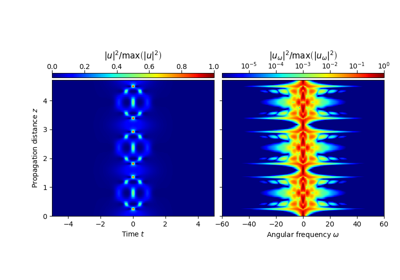
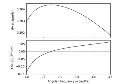
1.1. Basic examples
The step-by-step demonstrations in this gallery show how to perfom basic simulations using the provided software.


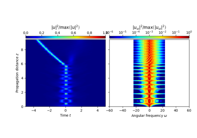
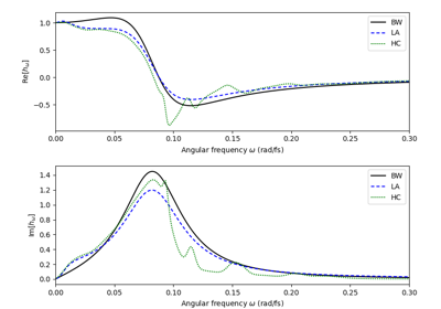
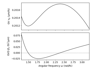
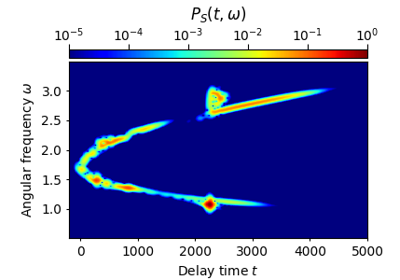
1.2. More specific examples
The step-by-step demonstrations in this gallery show how the functionality of the provided software can be used to customize the implemented models and to compute spectrograms.
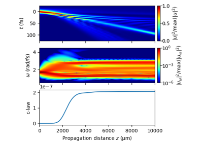
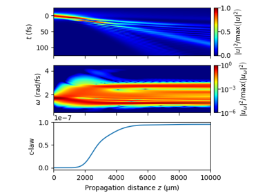
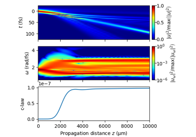
1.3. Photon number conservation
The examples provided in this gallery demonstrate the conservation of the photon number for the different models. Having available a proper conservation law is particularly important when the conservation quantity error method (CQE) is used for guiding step size adaption.
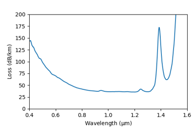
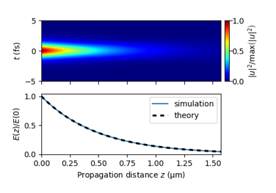
1.4. Attenuation
The examples provided in this gallery demonstrate how to use models that incorporate loss in terms of an absorption constant or a frequency dependent absorption profile.

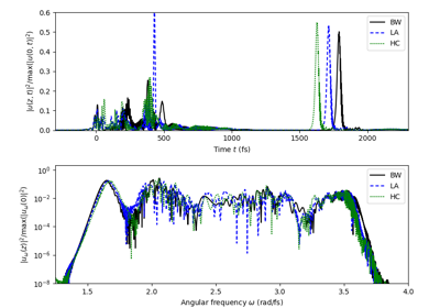
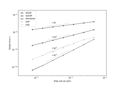
1.5. Performance tests
The step-by-step demonstrations in this gallery illustrate performance tests for the various implemented solver types. All test cases are implemented on basis of the standard nonlinear Schrödinger equation.
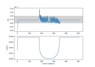
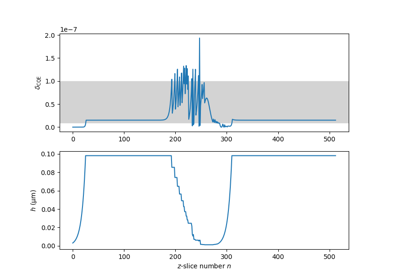
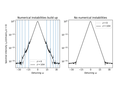
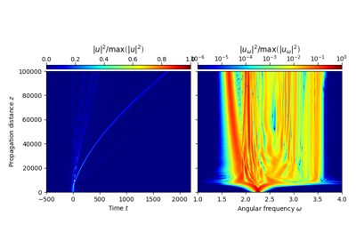
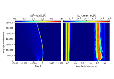
1.6. Propagation errors
The step-by-step demonstrations in this gallery demonstrate propagation errors that can occur when the computational domain does not properly support the intendet propagation scenario. We include these to assist users to identify possible error sources, and to raise awareness to ensure that the propagation \(z\)-increment is small enough, the computational domain is large enough, and to bear in mind the periodic boundary conditions along the time-axis. All test cases are implemented on basis of the standard nonlinear Schrödinger equation.