1.6.1. Implementing an anti-aliasing technique with a model

When performing nonlinear computations on discrete grids, it is important to choose the time window and the number of sample points large enough to prevent aliasing errors [B2001]. This example demonstrates how to implement an anti-aliasing technique directly with a model.

For a nonlinearity of order three, as for the cubic Kerr nonlinearity, an easy anti-aliasing procedure is to extend the spectrum by a factor of two and to proceed by zero-padding [HCL2008] [FCGK2005]. Therefore, in each step, after the nonlinear term is evaluated in the time domain and transformed to the Fourier domain, the upper half of the spectrum is set to zero.

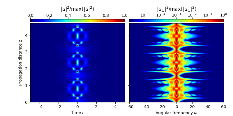
Here, the symmetric split-step Fourier method is used and the propagation of a fourth-order soliton is considered.

We first import the functionality needed to perform the sequence of numerical experiments:

import sys; sys.path.append('../../')
import numpy as np
import numpy.fft as nfft
from fmas.models import ModelBaseClass
from fmas.config import FTFREQ, FT, IFT, C0
from fmas.solver import  SySSM
from fmas.grid import Grid
from fmas.tools import plot_evolution

Next, we implement a model for the nonlinear Schrödinger equation. In particular, we here consider the standard nonlinear Schrödinger equation, given by

\[\partial_z u = -i \frac{\beta_2}{2}\partial_t^2 u + i\gamma |u|^2 u,\]

wherein \(u = u(z, t)\) represents the slowly varying pulse envelope, \(\beta_2=-1\) is the second order dispersion parameter, and \(\gamma=1\) is the nonlinear parameter. As discussed above, we here implement a simple technique allowing to compute the nonlinear term free of aliasing errors.

class NSE(ModelBaseClass):

    def __init__(self, w, b2 = -1.0, gamma = 1.):
        super().__init__(w, 0.5*b2*w*w)
        self.gamma = gamma
        # ANTI-ALIASING FILTER SETTING UPPER HALF OF SPECTRUM TO ZERO
        self._de_alias = lambda uw: np.where(np.abs(w) < 0.5 * w.max(), uw, 0j)

    @property
    def Lw(self):
        return 1j*self.beta_w

    def Nw(self, uw):
        ut = IFT(uw)
        return self._de_alias(1j*self.gamma*FT(np.abs(ut)**2*ut))

Next, we initialize the computational domain and use a symmetric split-step Fourier method to propagate a single third-order soliton for six soliton periods. For this numerical experiment, the extend of the time domain and the number of sample points is chosen large enough to allow for a zero padding anti-aliasing technique without cropping important parts of the spectrum.

grid = Grid( t_max = 34., t_num = 2**12)
t, w = grid.t, grid.w
model = NSE(w, b2=-1., gamma=1.)
u_0t = 4./np.cosh(t)

solver = SySSM(model.Lw, model.Nw)
solver.set_initial_condition(w, FT(u_0t))
solver.propagate(z_range = 3*np.pi/2, n_steps = 10000, n_skip = 50)
z, utz = solver.z_, solver.utz

plot_evolution( solver.z, grid.t, solver.utz,
    t_lim = (-5,5), w_lim = (-60,60), DO_T_LOG=False)

References:

B2001

J.P. Boyd, Chebychev and Fourier Spectral Methods, Dover, New York (2001)

HCL2008

H. Holmas, D. Clamond, H.P. Langtangen, A pseudospectral Fourier method for a 1D incompressible two-fluid model, Int. J. Numer. Meth. Fluids 58 (2008) 639, https://doi.org/10.1002/fld.1772

FCGK2005

D. Fuctus, D. Clamond, J. Grue, O. Kristiansen, An efficient model for three-dimensional surface wave simulations Part I: Free space problems, J. Comp. Phys. 205 (2005) 665, https://doi.org/10.1016/j.jcp.2004.11.027