1.6.2. Propagation errors caused by a too narrow frequency window

This example demonstrates that if the computational domain does not support the propagation scenario in an adequate manner, errors accumulate and results will give a wrong impression of the dynamics.

Here, the simple split-step Fourier method is used and the propagation of a third-order soliton is considered.

We first import the functionality needed to perform the sequence of numerical experiments:

import sys; sys.path.append('../../')
import numpy as np
import numpy.fft as nfft
from fmas.models import ModelBaseClass
from fmas.config import FTFREQ, FT, IFT, C0
from fmas.solver import SiSSM, SySSM, IFM_RK4IP, LEM_SySSM, CQE
from fmas.grid import Grid
from fmas.tools import plot_evolution

Next, we implement a model for the nonlinear Schrödinger equation. In particular, we here consider the standard nonlinear Schrödinger equation, given by

\[\partial_z u = -i \frac{\beta_2}{2}\partial_t^2 u + i\gamma |u|^2 u,\]

wherein \(u = u(z, t)\) represents the slowly varying pulse envelope, \(\beta_2=-1\) is the second order dispersion parameter, and \(\gamma=1\) is the nonlinear parameter:

class NSE(ModelBaseClass):

    def __init__(self, w, b2 = -1.0, gamma = 1.):
        super().__init__(w, 0.5*b2*w*w)
        self.gamma = gamma

    @property
    def Lw(self):
        return 1j*self.beta_w

    def Nw(self, uw):
        ut = IFT(uw)
        return 1j*self.gamma*FT(np.abs(ut)**2*ut)

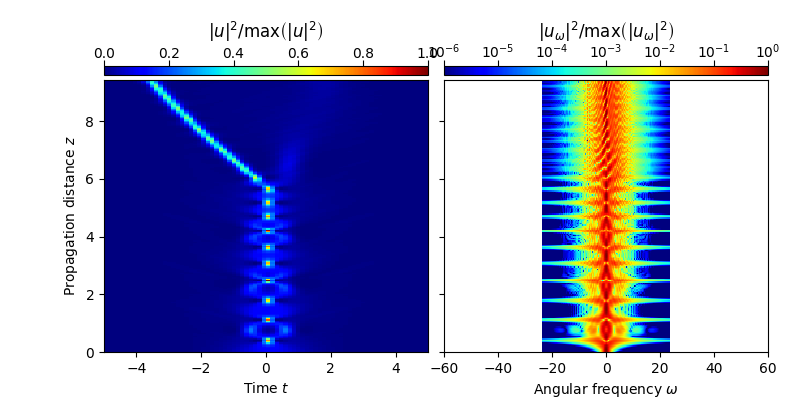
Next, we initialize the computational domain and use a simple split-step Fourier method to propagate a single third-order soliton for six soliton periods. In this first numerical experiment, the extend of the frequency domain is so small that, when the solitons spectrum broadens, it exceeds the bounds of the frequency domain. Errors stemming from truncation of the spectrum accumulate over subsequent soliton periods, giving an erroneous account of the true dynamics (see the subsequent figure).

# -- INITIALIZATION STAGE
# ... COMPUTATIONAL DOMAIN
grid = Grid( t_max = 34., t_num = 2**9)
t, w = grid.t, grid.w

# ... NSE MODEL
model = NSE(w, b2=-1., gamma=1.)
# ... INITIAL CONDITION
u_0t = 3./np.cosh(t)


solver = SiSSM(model.Lw, model.Nw)
solver.set_initial_condition(w, FT(u_0t))
solver.propagate(z_range = 6*np.pi/2, n_steps = 10000, n_skip = 50)
z, utz = solver.z_, solver.utz

plot_evolution( solver.z, grid.t, solver.utz,
    t_lim = (-5,5), w_lim = (-60,60), DO_T_LOG=False)

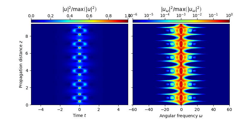
In the subsequent numerical experiment, the extend of the frequency domain is increased to fully support the third-order soliton in those propagation stages where its spectrum is maximally broad. As a result, the periodic dynamics of the higher order soliton is well represented (see the subsequent figure).

grid = Grid( t_max = 34., t_num = 2**11)
t, w = grid.t, grid.w
model = NSE(w, b2=-1., gamma=1.)
u_0t = 3./np.cosh(t)


solver = SiSSM(model.Lw, model.Nw)
solver.set_initial_condition(w, FT(u_0t))
solver.propagate(z_range = 6*np.pi/2, n_steps = 10000, n_skip = 50)
z, utz = solver.z_, solver.utz

plot_evolution( solver.z, grid.t, solver.utz,
    t_lim = (-5,5), w_lim = (-60,60), DO_T_LOG=False)