1.6.3. Numerical instabilities of the Nonlinear Schrödinger Equation

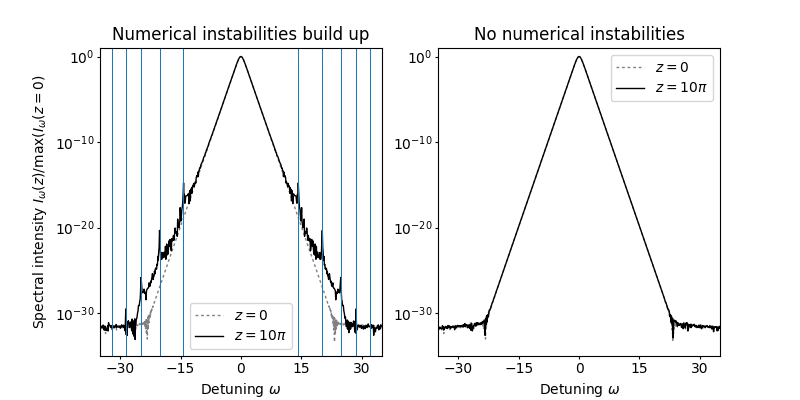
This example demonstrates numerical instabilities that build up during simulations of the standard nonlinear Schrödinger equation when the \(z\)-increment used for propagtion is too small.

Here, the simple split-step Fourier method is used and the instabilities develop from round-off errors during the propagation of a fundamental soliton.

The numerical instabilities of the nonlinear Schrödinger equation developing on top of plain wave solutions where first studied in Ref. [WH1986]. An in-depth study of instabilities of the split-step Fourier method for the simulation of the nonlinear Schrödinger equation, developing on a background given by a soliton, is provided by Ref. [L2012].

We first import the functionality needed to perform the sequence of numerical experiments:

import sys
import numpy as np
import numpy.fft as nfft
from fmas.models import ModelBaseClass
from fmas.config import FTFREQ, FT, IFT, C0
from fmas.solver import SiSSM, SySSM, IFM_RK4IP, LEM_SySSM, CQE
from fmas.grid import Grid

Next, we implement a model for the nonlinear Schrödinger equation. In particular, we here consider the standard nonlinear Schrödinger equation, given by

\[\partial_z u = -i \frac{\beta_2}{2}\partial_t^2 u + i\gamma |u|^2 u,\]

wherein \(u = u(z, t)\) represents the slowly varying pulse envelope, \(\beta_2=-1\) is the second order dispersion parameter, and \(\gamma=1\) is the nonlinear parameter:

class NSE(ModelBaseClass):

    def __init__(self, w, b2 = -1.0, gamma = 1.):
        super().__init__(w, 0.5*b2*w*w)
        self.gamma = gamma

    @property
    def Lw(self):
        return 1j*self.beta_w

    def Nw(self, uw):
        ut = IFT(uw)
        return 1j*self.gamma*FT(np.abs(ut)**2*ut)

Next, we initialize the computational domain and use a simple split-step Fourier method to propagate a single fundamental soliton for ten soliton periods.

# -- INITIALIZATION STAGE
# ... COMPUTATIONAL DOMAIN
grid = Grid( t_max = 30., t_num = 2**10)
t, w = grid.t, grid.w
# ... NSE MODEL
model = NSE(w, b2=-1., gamma=1.)
# ... INITIAL CONDITION
u_0t = 1./np.cosh(t)

In a first numerical experiment, the stepsize is intentionally kept very large in order to allow the numerical istabilities to build up.

solver = SySSM(model.Lw, model.Nw)
solver.set_initial_condition(w, FT(u_0t))
solver.propagate(z_range = 10*np.pi, n_steps = 511, n_skip = 1)
z, utz = solver.z_, solver.utz

In this case, instabilities are expected to build up since the \(z\)-increment \(\Delta z\), used by the propagation algorithm, exceeds the threshold increment \(\Delta z_{\mathrm{T}}=2\pi/\mathrm{max}(\omega)\) (both increments are displayed below).

# -- MAXIMUM FREQUENCY SUPPORTED ON COMPUTATIONAL GRID
w_max = np.pi/(t[1]-t[0])
# -- THRESHOLD INCREMENT
dz_T = np.pi*2/w_max**2

print("Increment dz =", z[1]-z[0])
print("Threshold increment dz_T =", dz_T)

Out:

Increment dz = 0.061479308289428436
Threshold increment dz_T = 0.0021856605344040803

In a second numerical experiment, the stepsize is set small enough to shift the resonance outside the computational domain.

solver = SySSM(model.Lw, model.Nw)
solver.set_initial_condition(w, FT(u_0t))
solver.propagate(z_range = 10*np.pi, n_steps = 15000, n_skip = 1)
z2, utz2 = solver.z_, solver.utz

print("Increment dz =", z2[1]-z2[0])
print("Threshold increment dz_T =", dz_T)

Out:

Increment dz = 0.0020943951023931952
Threshold increment dz_T = 0.0021856605344040803

Next, we prepare a figure that shows the results of the above to experiments. The left subfigure shows the results of the first simulation run in which the numerical instabilities and their predicted locations are shown. The right subfigure shows the results of second simulation run in which the \(z\)-increment was small enough to shift the instabilities outside the computational domain.

import matplotlib as mpl
import matplotlib.pyplot as plt
import matplotlib.colors as col

f, (ax,ax2) = plt.subplots(1, 2, figsize=(8,4))

# -- EXAMPLE WITH INSTABILITIES

dz = z[1]-z[0]
w_I = lambda n: np.sqrt(n*2*np.pi*2./dz)

shift=nfft.fftshift
Iw_ini = np.abs(FT(utz[0]))**2
Iw_fin = np.abs(FT(utz[-1]))**2
ax.plot(shift(w), shift(Iw_ini)/np.max(Iw_ini), color='gray', dashes=[2,2], lw=1., label='$z=0$')
ax.plot(shift(w), shift(Iw_fin)/np.max(Iw_ini), color='k', lw=1., label='$z=10\pi$')

for n in range(1,20,1):
    ax.axvline(w_I(n), lw=0.75)
    ax.axvline(-w_I(n), lw=0.75)

dw_lim = (-35,35)
dw_ticks = (-30, -15, 0, 15, 30)
ax.tick_params(axis='x', length=2., pad=2, top=False)
ax.set_xlim(dw_lim)
ax.set_xticks(dw_ticks)
ax.set_xlabel(r"Detuning $\omega$")

y_lim = (1e-35,10)
y_ticks = (1e-30,1e-20,1e-10,1)
ax.tick_params(axis='y', length=2., pad=2, top=False)
ax.set_yscale('log')
ax.set_ylim(y_lim)
ax.set_yticks(y_ticks)
ax.set_ylabel(r"Spectral intensity $I_\omega(z)/\mathrm{max}(I_\omega(z=0)}$")
ax.set_title(r"Numerical instabilities build up")

ax.legend()

# -- EXAMPLE WITHOUT INSTABILITIES

Iw_ini = np.abs(FT(utz2[0]))**2
Iw_fin = np.abs(FT(utz2[-1]))**2
ax2.plot(shift(w), shift(Iw_ini)/np.max(Iw_ini), color='gray', dashes=[2,2], lw=1., label='$z=0$')
ax2.plot(shift(w), shift(Iw_fin)/np.max(Iw_ini), color='k', lw=1., label='$z=10\pi$')

ax2.tick_params(axis='x', length=2., pad=2, top=False)
ax2.set_xlim(dw_lim)
ax2.set_xticks(dw_ticks)
ax2.set_xlabel(r"Detuning $\omega$")

ax2.tick_params(axis='y', length=2., pad=2, top=False)
ax2.set_yscale('log')
ax2.set_ylim(y_lim)
ax2.set_yticks(y_ticks)
ax2.set_title(r"No numerical instabilities")

ax2.legend()

plt.show()

References:

WH1986

J.A.C. Weideman, B.M. Herbst, Split-step methods for the solution of the nonlinear Schrödinger equation, SIAM J. Numer. Anal., 23 (1986) 485, http://www.jstor.org/stable/2157521.

L2012

T.I. Lakoba, Instability Analysis of the Split-Step Fourier Method on the Background of a Soliton of the Nonlinear Schrödinger Equation, Numerical Methods for Partial Differential Equations 28 (2012) 641, https://doi.org/10.1002/num.20649