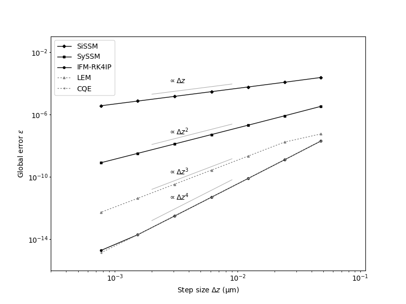
1.5.3. Scaling behavior of global errors

This example demonstrates the accuracy of the various \(z\)-propagation algorithms. As test case, the propagation dynamics of a fundamental soliton in terms of the standard nonlinear Schrödinger equation is considered. For this particular case, an exact solution is available to which a numerical approximation can be compared to.

We first import the functionality needed to perform the sequence of numerical experiments:

import sys
import numpy as np
import numpy.fft as nfft
from fmas.models import ModelBaseClass
from fmas.config import FTFREQ, FT, IFT, C0
from fmas.solver import SiSSM, SySSM, IFM_RK4IP, LEM_SySSM, CQE
from fmas.grid import Grid

Next, we implement a model for the nonlinear Schrödinger equation. In particular, we here consider the standard nonlinear Schrödinger equation, given by

\[\partial_z u = -i \frac{\beta_2}{2}\partial_t^2 u + i\gamma |u|^2 u,\]

wherein \(u = u(z, t)\) represents the slowly varying pulse envelope, \(\beta_2=-1\) is the second order dispersion parameter, and \(\gamma=1\) is the nonlinear parameter:

class NSE(ModelBaseClass):

    def __init__(self, w, b2 = -1.0, gamma = 1.):
        super().__init__(w, 0.5*b2*w*w)
        self.gamma = gamma

    @property
    def Lw(self):
        return 1j*self.beta_w

    def Nw(self, uw):
        ut = IFT(uw)
        return 1j*self.gamma*FT(np.abs(ut)**2*ut)

Next, we implement a function that performs a single numerical experiment, in which a single fundamental soliton is propagated for a specified distance.

The exact single-soliton solution of the above nonlinar Schrödinger equation is given by

\[u_{\rm{exact}}(z,t) = \sqrt{P_0} {\rm{sech}}(t/t_0)\,e^{-i\gamma P_0 z/2},\]

with \(P_0=|\beta_2|/(\gamma t_0^2)\). We here consider a fundamental soliton of duration \(t_0=1\) and use \(u_{\rm{exact}}(0,t)\) as initial condition. The propagation is performed up to \(z_{\rm{max}}=\pi/2\), i.e. for one soliton period.

The function below performs a parameter sweep over a range of step sizes \(\Delta z\), and compares the approximate solution \(u(z_{\rm{max}},t)\) at the final position, obtained for a specified \(z\)-propagation algorithm, to the exact solution \(u_{\rm{exact}}(z_{\rm{max}},t)\) at that point. This is done by computing the average relative intensity error, given by

\[\epsilon = \frac{ \int \left| |u(z_{\rm{max}},t)|^2 - |u_{\rm{exact}}(z_{\rm{max}},t)|^2 \right|\,{\rm{d}}t}{ \int P_0 {\rm{d}}t}\]

This error measure was also used in [H2007] to compare the performance of different \(z\)-propagation algorithms. The function then returns the sequence of step sizes and the corresponding error values:

def determine_error(mode):

    # -- SET AXES
    grid = Grid( t_max = 50., t_num = 2**12)
    t, w = grid.t, grid.w

    # -- INITIALIZATION STAGE
    # ... SET MODEL
    b2 = -1.
    gamma = 1.
    model = NSE(w, b2, gamma)
    # ... SET SOLVER TYPE
    switcher = {
        'SiSSM': SiSSM(model.Lw, model.Nw),
        'SySSM': SySSM(model.Lw, model.Nw),
        'IFM': IFM_RK4IP(model.Lw, model.Nw),
        'LEM': LEM_SySSM(model.Lw, model.Nw),
        'CQE': CQE(model.Lw, model.Nw, del_G=1e-6)
    }
    try:
        my_solver = switcher[mode]
    except KeyError:
        print('NOTE: MODE MUST BE ONE OF', list(switcher.keys()))
        raise
        exit()

    # -- AVERAGE RELATIVE INTENSITY ERROR
    _RI_error = lambda x,y: np.sum(np.abs(np.abs(x)**2-np.abs(y)**2)/x.size/np.max(np.abs(y)**2))

    # -- SET TEST PULSE PROPERTIES (FUNDAMENTAL SOLITON)
    t0 = 1.                       # duration
    P0 = np.abs(b2)/t0/t0/gamma   # peak-intensity
    LD = t0*t0/np.abs(b2)         # dispersion length
    # ... EXACT SOLUTION
    u_exact = lambda z, t: np.sqrt(P0)*np.exp(0.5j*gamma*P0*z)/np.cosh(t/t0)
    # ... INITIAL CONDITION FOR PROPAGATION
    u0_t = u_exact(0.0, t)

    res_dz = []
    res_err = []
    for z_num in [2**n for n in range(5,12)]:
        # ...  PROPAGATE INITIAL CONITION
        my_solver.set_initial_condition(w, FT(u0_t))
        my_solver.propagate(
                z_range = 0.5*np.pi*LD,
                n_steps = z_num,
                n_skip = 8
                )

        # ... KEEP RESULTS
        z_fin = my_solver.z[-1]
        dz =  z_fin/(z_num+1)
        u_t_fin = my_solver.utz[-1]
        u_t_fin_exact = u_exact(z_fin, t)
        res_dz.append(dz)
        res_err.append(_RI_error( u_t_fin, u_t_fin_exact))

        # ... CLEAR DATA FIELDS
        my_solver.clear()

    return np.asarray(res_dz), np.asarray(res_err)

Finally, we prepare a figure that shows the scaling behavior of the resulting relative intensity error for the different propagation algorithms side-by-side:

import matplotlib as mpl
import matplotlib.pyplot as plt
import matplotlib.colors as col

f, ax = plt.subplots(1, 1, figsize=(8,6))

col1 = col12 = 'k'

dz, err = determine_error("SiSSM")
l1 = ax.plot(dz, err, color=col1, marker='D', markersize=3., markerfacecolor=col1, linewidth=1, label=r'SiSSM')

dz, err = determine_error("SySSM")
l2 = ax.plot(dz, err, color=col1, marker='s', markersize=3., markerfacecolor=col12, linewidth=1., label=r'SySSM')

dz, err = determine_error("IFM")
l3 = ax.plot(dz, err, color=col1, marker='o', markersize=3., markerfacecolor=col12, linewidth=1., label=r'IFM-RK4IP')

col1 = col12 = 'gray'

dz, err = determine_error("LEM")
l4 = ax.plot(dz, err, color=col1, marker='^', markersize=3., markerfacecolor=col12, linewidth=1., dashes=[2,2], mew = 1., label=r'LEM')

dz, err = determine_error("CQE")
l5 = ax.plot(dz, err, color=col1, marker='<', markersize=2., markerfacecolor=col12, linewidth=1., mew= 1., dashes=[2,2], label=r'CQE')

ax.legend()

line = lambda a, b, x: a*x**b
dz_ = np.linspace(2e-3,9e-3,5)
ax.plot(dz_, line(0.010, 1, dz_), linewidth=0.75, color='darkgray')
ax.plot(dz_, line(0.003, 2, dz_), linewidth=0.75, color='darkgray')
ax.plot(dz_, line(0.002, 3, dz_), linewidth=0.75, color='darkgray')
ax.plot(dz_, line(0.01, 4, dz_), linewidth=0.75, color='darkgray')

ax.text( 0.375, 0.80, r'$\propto \Delta z$', transform=ax.transAxes)
ax.text( 0.375, 0.58, r'$\propto \Delta z^2$', transform=ax.transAxes)
ax.text( 0.375, 0.41, r'$\propto \Delta z^3$', transform=ax.transAxes)
ax.text( 0.375, 0.30, r'$\propto \Delta z^4$', transform=ax.transAxes)

dz_lim = (3e-4,0.11)
dz_ticks = (1e-3, 1e-2, 1e-1)
ax.tick_params(axis='x', length=2., pad=2, top=False)
ax.set_xscale('log')
ax.set_xlim(dz_lim)
ax.set_xticks(dz_ticks)
ax.set_xlabel(r"Step size $\Delta z~\mathrm{(\mu m)}$")

err_lim = (0.1e-15,1e-1)
err_ticks = (1e-14,1e-10,1e-6,1e-2)
ax.tick_params(axis='y', length=2., pad=2, top=False)
ax.set_yscale('log')
ax.set_ylim(err_lim)
ax.set_yticks(err_ticks)
ax.set_ylabel(r"Global error $\epsilon$")

plt.show()

References:

H2007

J. Hult, A Fourth-Order Runge–Kutta in the Inter- action Picture Method for Simulating Supercontin- uum Generation in Optical Fibers, IEEE J. Light- wave Tech. 25 (2007) 3770, https://doi.org/10.1109/JLT.2007.909373.