1.5.2. Stepsize adaption in the CQE method

This example demonstrates the ability of the conservation quantity error (CQE) method [H2009] to locally decrease the stepsize when higher accuracy is needed. As test case, the interaction dynamics of two colliding fundamental soliton governed by the standard nonlinear Schrödinger equation is considered.

In contrast to the LEM, which uses a local error derived by means of step-doubling and extrapolation, the CQE uses a conservation quantity of the underlying propagation equation to drive stepsize adaption.

We first import the functionality needed to perform the sequence of numerical experiments:

import sys
import numpy as np
from fmas.models import ModelBaseClass
from fmas.config import FTFREQ, FT, IFT, C0
from fmas.grid import Grid
from fmas.solver import CQE
from fmas.data_io import save_h5
from fmas.tools import plot_evolution

Next, we implement a model for the nonlinear Schrödinger equation. In particular, we here consider the standard nonlinear Schrödinger equation, given by

\[\partial_z u = -i \frac{\beta_2}{2}\partial_t^2 u + i\gamma |u|^2 u,\]

wherein \(u = u(z, t)\) represents the slowly varying pulse envelope, \(\beta_2=-1\) is the second order dispersion parameter, and \(\gamma=1\) is the nonlinear parameter:

class NSE(ModelBaseClass):

    def __init__(self, w, beta, gamma):
        super().__init__(w, beta_w=beta)
        self.gamma = gamma

    @property
    def Lw(self):
        return 1j*self.beta_w

    def N(self, uw):
        ut = IFT(uw)
        return 1j*self.gamma*FT(np.abs(ut)**2*ut)

Next, we set up the computational domain, the model, and the LEM solver and prepare an initial condition with two fundamental solitons. The velocity of the solitons is adjusted so that they collide after approximately half a soliton period.

To construct the initial condition, we use the exact single-soliton solution of the nonlinar Schrödinger equation, given by

\[u_{\rm{exact}}(z,t) = \sqrt{P_0} {\rm{sech}}(t/t_0)\,e^{-i\gamma P_0 z/2},\]

with \(P_0=|\beta_2|/(\gamma t_0^2)\). We here consider two fundamental solitons of duration \(t_0=1\) and frequency detunings \(\omega_0=25\) to construct the initial condition

The propagation is performed up to \(z_{\rm{max}}=\pi/2\), i.e. for one soliton period.

# -- SET MODEL PARAMETERS
t_max = -50.
Nt = 2**12
# ... PROPAGATION CONSTANT (POLYNOMIAL MODEL)
beta = np.poly1d([-0.5, 0.0, 0.0])
beta1 = np.polyder(beta, m=1)
beta2 = np.polyder(beta, m=2)
# ... NONLINEAR PARAMETER
gamma = 1.
# ... SOLITON PARAMTERS
t0 = 1.                             # duration
t_off = 20.                         # temporal offset
w0 = 25.                            # detuning
P0 = np.abs(beta2(0))/t0/t0/gamma   # peak-intensity
LD = t0*t0/np.abs(beta2(0))         # dispersion length
# ... EXACT SOLUTION
u_exact = lambda z, t: np.sqrt(P0)*np.exp(0.5j*gamma*P0*z)/np.cosh(t/t0)

# -- INITIALIZATION STAGE
# ... COMPUTATIONAL DOMAIN
grid = Grid(t_max=t_max, t_num=Nt)
t, w = grid.t, grid.w
# ... NONLINEAR SCHROEDINGER EQUATION
model = NSE(w, beta(w), gamma)
# ... PROPAGATION ALGORITHM

In order to drive stepsize adaption, the CQE method monitors a conservation law exhibited by the underlying propagation equation. Here, for the standard nonlinear Schrödinger equation, we opt to use the conserved quantity

implemented by the function:

def my_CQE_fun(i, zi, w, uw):
    return np.sum(np.abs(uw)**2)

The function can be set when an instance of the solver is initialized:

solver = CQE(model.Lw, model.N, del_G = 1e-7, user_action = my_CQE_fun)
# ... INITIAL CONDITION
u0_t  = u_exact(0.0, t+t_off)*np.exp(1j*w0*t)
u0_t += u_exact(0.0, t-t_off)*np.exp(-1j*w0*t)
solver.set_initial_condition(w, FT(u0_t))

# -- RUN SOLVER
solver.propagate(
    z_range = 0.5*np.pi*LD,     # propagation range
    n_steps = 512,
    n_skip = 2
)

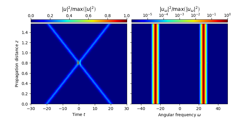
The figure below shows the propagation dynamics of the above initial condition:

plot_evolution( solver.z, grid.t, solver.utz, t_lim = (-30,30), w_lim = (-50.,50.))

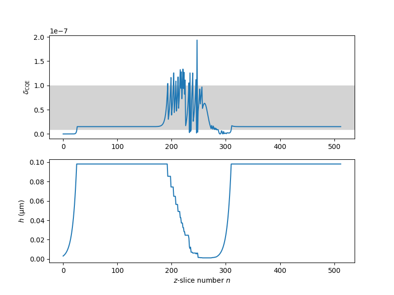
Below we prepare a figure showing the variation of the local relative error upon propagation (top figure), and the decrease of the local stepsize in the vicinity of the soliton-soliton collision (bottom subfigure). In the top figure, the shaded region indicates the local goal error range. Aim of the CQE method is to keep the conservation quantity error within that range.

# sphinx_gallery_thumbnail_number = 2

import matplotlib as mpl
import matplotlib.pyplot as plt
import matplotlib.colors as col

f, (ax1,ax2) = plt.subplots(2, 1, figsize=(8,6))

ax1.plot(range(len(solver._del_rle)), solver._del_rle)
ax1.axhspan(0.1e-7,1e-7,color='lightgray')
ax1.set_ylabel(r"$\delta_{\rm{CQE}}$")

ax2.plot(range(len(solver._dz_a)), solver._dz_a)
ax2.set_ylabel(r"$h~{(\mathrm{\mu m})}$")
ax2.set_xlabel(r"$z$-slice number $n$")

plt.show()

References:

H2009

A. M. Heidt, Efficient Adaptive Step Size Method for the Simulation of Supercontinuum Generation in Optical Fibers, IEEE J. Lightwave Tech. 27 (2009) 3984, https://doi.org/10.1109/JLT.2009.2021538