1.3.3. FMAS

This example demonstrates photon number conservation for the forward model for the analytic signal (FMAS).

The considered propagation model provides a proper conservation law as class method claw. However, for clarity, we here re-implement the conservation law and explicitly pass this user-defined function to the solver class upon initialization.

As exemplary propagation scenario, the setup used in the step-by-step demo

Computing spectrograms

is used.

import fmas
import numpy as np
from fmas.solver import IFM_RK4IP
from fmas.analytic_signal import AS
from fmas.grid import Grid
from fmas.propagation_constant import PropConst, define_beta_fun_ESM
from fmas.tools import sech, change_reference_frame, plot_claw

beta_fun = define_beta_fun_ESM()
pc = PropConst(beta_fun)

grid = Grid(t_max=5500.0, t_num=2 ** 14)  # (fs)  # (-)

Ns = 8.0  # (-)
t0 = 7.0  # (fs)
w0 = 1.7  # (rad/fs)
n2 = 3.0e-8  # (micron^2/W)
chi = 8.0 * n2 * pc.beta(w0) * pc.c0 / w0 / 3.0
gam0 = 3 * w0 * w0 * chi / (8 * pc.c0 * pc.c0 * pc.beta(w0))
A0 = Ns * np.sqrt(abs(pc.beta2(w0)) / gam0) / t0
E_0t_fun = lambda t: np.real(A0 * sech(t / t0) * np.exp(1j * w0 * t))
Eps_0w = AS(E_0t_fun(grid.t)).w_rep

As model we here consider the forward model for the analytic signal (FMAS)

from fmas.models import FMAS
model = FMAS(w=grid.w, beta_w=pc.beta(grid.w), chi=chi)

For the FMAS \(z\)-propagation model we consider a conserved quantity that is related to the classical analog of the photon number, see Eq. (24) of Ref. [AD2010] below. In particular we here implement

\[C_p(z) = \sum_{\omega>0} \omega^{-2} \beta(\omega) |u_\omega(z)|^2,\]

which is, by default, provided as method model.claw .

beta_w = pc.beta(grid.w)  # pre-compute beta(w) for convenience


def Cp(i, zi, w, uw):
    _a2_w = np.divide(
        np.abs(beta_w) * np.abs(uw) ** 2,
        w * w,
        out=np.zeros(w.size, dtype="float"),
        where=w > 0,
    )
    return np.sum(_a2_w)

As shown below, this conserved quantity can be provided when an instance of the desired solver is initialized. Here, for simply monitoring the conservation law we use the Runge-Kutta in the ineraction picture method. However, a proper conserved quantity is especially important when the conservation quantity error method (CQE) is used, see, e.g., demo

Stepsize adaption in the CQE method

solver = IFM_RK4IP(model.Lw, model.Nw, user_action=Cp)
solver.set_initial_condition(grid.w, Eps_0w)
solver.propagate(z_range=0.01e6, n_steps=4000, n_skip=8)  # (micron)  # (-)  # (-)

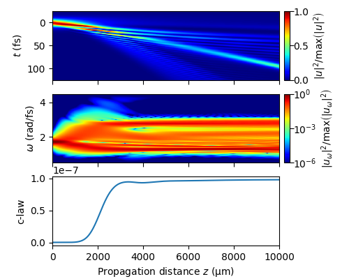
The figure below shows the dynamic evolution of the pulse in the time domain (top subfigure) and in the frequency domain (center subfigure). The subfigure at the bottom shows the conservation law (c-law) given by the normalized photon number variation

\[\delta_{\rm{Ph}}(z) = \frac{ C_p(z)-C_p(0)}{C_p(0)}\]

as function of the proapgation coordinate \(z\). For the considered discretization of the computational domain the normalized photon number variation is of the order \(\delta_{\rm{Ph}}\approx 10^{-7}\) and thus very small. The value can be still decreased by decreasing the stepsize \(\Delta z\).

utz = change_reference_frame(solver.w, solver.z, solver.uwz, pc.vg(w0))

plot_claw(
    solver.z, grid.t, utz, solver.ua_vals, t_lim=(-25, 125), w_lim=(0.5, 4.5)
)

References:

[AD2010] Sh. Amiranashvili, A. Demircan, Hamiltonian structure of propagation equations for ultrashort optical pulses, Phys. Rev. E 10 (2010) 013812, http://dx.doi.org/10.1103/PhysRevA.82.013812.