1.2.4. Computing spectrograms

This examples shows how to use the simple spectrogram-tool provided the py-fmas package.

import fmas
import numpy as np
from fmas.models import FMAS_S_Raman
from fmas.solver import IFM_RK4IP
from fmas.analytic_signal import AS
from fmas.grid import Grid
from fmas.propagation_constant import PropConst
from fmas.tools import sech, plot_details_prop_const
from fmas.tools import change_reference_frame, plot_evolution
from fmas.tools import plot_spectrogram, spectrogram

Below we will demonstrate how to construct simple spectrograms using functions that are implemente in py-fmas.

We will first perform a simulation run for a short intense pulse, launched in the anomalous dispersion domain of an “endlessly single mode” (ESM) photonic crystal fiber [3]. The considered propagation scenario reproduces that of Ref. [1]. After the \(z\)-propagation algorithm completes, we will perform some data postprocessing. Specifically, we we will illustrate the time-frequency characteristics of the evolved scenario and point out a few points to bear in mind when constructing spectrograms.

The propagation constant of the ESM that we will use for the \(z\)-propagation simulation is given by

def define_beta_fun_ESM():
    r"""Custom propagation constant for an ESM photonic crystal fiber.

    Implements rational Pade-approximant of order [8/8] for the refractive
    index of a endlessly single mode (ESM) nonlinear photonic crystal fiber
    (PCF), see Ref. [1].

    References:
        [1] Visibly 'white' light generation in uniform photonic crystal fiber
        using a microchip laser Stone, J.M. and Knight, J.C.  Optics Express 16
        (2007) 2670.

    Returns:
        :obj:`callable`: Propagation constant for ESM PCF.
    """
    p = np.poly1d(
        (16.89475, 0., -319.13216, 0., 34.82210, 0., -0.992495, 0., 0.0010671)[::-1])
    q = np.poly1d(
        ( 1.00000, 0., -702.70157, 0., 78.28249, 0., -2.337086, 0., 0.0062267)[::-1])
    n_idx = lambda w: 1+p(w)/q(w) # (-)
    c0 = 0.29979                    # (micron/fs)
    return lambda w: n_idx(w)*w/c0  # (1/micron)

In order to prepare the propagation scenario, we first initialize the propagation constant and generate an instance of the PropConst convenience class.

beta_fun = define_beta_fun_ESM()
pc = PropConst(beta_fun)

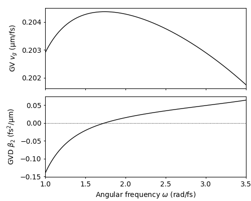
The group-velocity (GV) and group-velocity dispersion (GVD) of the ESM propagation constant in the angular frequency range \(\omega \in [1.2,3.2]~\mathrm{rad/fs}\) can then be visualized using build in py-fmas functions. GV and GVD are implemented by the class methods vg, and beta2, respectively. To generate a quick plot of both, we use the function plot_details_prop_const, which is defined in module tools.

w_tmp = np.linspace(1., 3.5, 400)
plot_details_prop_const(w_tmp, pc.vg(w_tmp), pc.beta2(w_tmp))

We next define the simulation parameters that specify the computational domain

grid = Grid(
    t_max = 5500.,  # (fs)
    t_num = 2**14   # (-)
)

After the computational domain is specified, we define the simulation parameters that are needed to specify the \(z\)-propagation model. Below, we use the simplified forward model for the analytic signal including the Raman effect [3]

model = FMAS_S_Raman(
    w=grid.w,
    beta_w = pc.beta(grid.w),
    n2= 3.0e-8      # (micron^2/W)
)

Thereafter, we speficy the initial condition. Here, we consider a single soliton with duration \(t_0=7\,\mathrm{fs}\) (i.e. approx. 3.8 cycles), center frequency \(\omega_0=1.7\,\mathrm{rad/fs}\), and soliton order \(N_{\rm{S}}=8\).

Ns = 8.0            # (-)
t0 = 7.0            # (fs)
w0 = 1.7            # (rad/fs)
A0 = Ns*np.sqrt(abs(pc.beta2(w0))*model.c0/w0/model.n2)/t0
E_0t_fun = lambda t: np.real(A0*sech(t/t0)*np.exp(1j*w0*t))

Above, the initial condition is prepared in the time-domain. Below we show how the frequency-domain representation of the analytic signal for use with one of the implemented \(z\)-propagation algorithms can be obtained:

Eps_0w =  AS(E_0t_fun(grid.t)).w_rep

For \(z\)-propagation we here use a variant of an integrating factor method, referred to as the “Runge-Kutta in the interaction picture” method, implemented as IFM_RK4IP in module solver.

solver = IFM_RK4IP( model.Lw, model.Nw)
solver.set_initial_condition( grid.w, Eps_0w)
solver.propagate(
    z_range = 0.12e6,   # (micron)
    n_steps = 2000,     # (-)
    n_skip = 10         # (-)
)

Once the \(z\)-propagation algorithm terminates we can perform a shift to a frame of reference in which the initial pulse is stationary, i.e. to a moving frame of reference with velocity \(v_0=v_g(\omega_0)\). The evolution of the analytic signal can then be visualized using the function plot_evolution defined in module tools:

utz = change_reference_frame(solver.w, solver.z, solver.uwz, pc.vg(w0))
plot_evolution( solver.z, grid.t, utz, t_lim=(-200,2500), w_lim=(0.6,3.4))

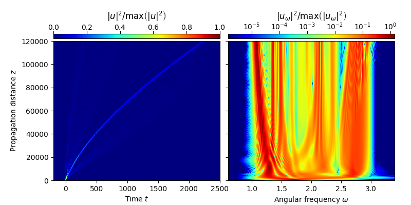
This reproduces Fig. 1 of Ref. [1].

Analytic signal spectrograms that show the time-frequency characteristics of the field can be constructed using the function spectrogram defined in module tools. These spectrograms are computed by using a Gaussian function for localizing the analytic signal along the time-axis. The root-mean-square (rms) width of this window-function needs to be chosen carefully, as demonstrated below. Consider, e.g., the propagation distance \(z=0.12~\mathrm{m}\), for which the analytic signal can be obtained as

z0_idx = np.argmin(np.abs(solver.z-0.12e6))
Et = utz[z0_idx]

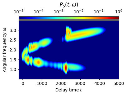
Using a very small rms-width \(s_0=10~\mathrm{fs}\) for the window-function results in a distorted spectrogram. The temporal resolution is good, but the frequency resolution is quite bad (cf. Fig. 2(a) of Ref. [1]):

tau, w, P = spectrogram(grid.t,grid.w,Et,t_lim=(-200.,5000.),Nt=600,Nw=512,s0=10.)
w_mask = np.logical_and(w>0.5,w<3.5)
plot_spectrogram(tau, w[w_mask], P[w_mask])

Using a very large rms-width \(s_0=140~\mathrm{fs}\) also results in a distorted spectrogram. This time the frequency resolution is good, but the temporal resolution is bad (cf. Fig. 2(b) of Ref. [1]):

tau, w, P = spectrogram(grid.t,grid.w,Et,t_lim=(-200.,5000.),Nt=600,Nw=512,s0=140.)
w_mask = np.logical_and(w>0.5,w<3.5)
plot_spectrogram(tau, w[w_mask], P[w_mask])

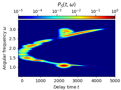
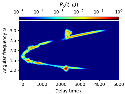
For this particular example, an optimal time-frequency resolution is achieved for the rms-width \(s_0=39.1~\mathrm{fs}\). This value was obtained using the optfrog Python tool, see Ref. [1] below. We here simply use this rms-width with the simple spectrogram implemented along with py-fmas (cf. Fig. 2(c) of Ref. [1]):

tau, w, P = spectrogram(grid.t,grid.w,Et,t_lim=(-200.,5000.),Nt=600,Nw=512,s0=39.1)
w_mask = np.logical_and(w>0.5,w<3.5)
plot_spectrogram(tau, w[w_mask], P[w_mask])

# sphinx_gallery_thumbnail_number = 5

Finally, let us note that the functionality of py-fmas can be extended by the optfrog tool in a straight-forward manner. In fact, optfrog was specifically written for use with py-fmas. An example that shows how to use py-fmas along with optfrog is shown under the link below:

Extending py-fmas by optfrog spectrograms

References:

[1] O. Melchert, B. Roth, U. Morgner, A. Demircan, OptFROG — Analytic signal spectrograms with optimized time–frequency resolution, SoftwareX 10 (2019) 100275, https://doi.org/10.1016/j.softx.2019.100275, code repository: https://github.com/ElsevierSoftwareX/SOFTX_2019_130.

[2] J. M. Stone, J. C. Knight, Visibly ‘white’ light generation in uniform photonic crystal fiber using a microchip laser, Optics Express 16 (2007) 2670.

[3] A. Demircan, Sh. Amiranashvili, C. Bree, C. Mahnke, F. Mitschke, G. Steinmeyer, Rogue wave formation by accelerated solitons at an optical event horizon, Appl. Phys. B 115 (2014) 343, http://dx.doi.org/10.1007/s00340-013-5609-9