1.2.3. Using the PropConst convenience class

This example demonstrates how the PropConst class, implemented in module fmas.propagation_constant, can be used to wrap and analyse a user supplied propagation constant.

The use of this class is optional. py-fmas can be used without this class. However, this class makes it convenient to display and analyze a given propagation constant. In order to use PropConst, the propagation constant needs to be available as a callable function.

We first start by importing the functionality of numpy and fmas into the current namespace. In particular, we also import the convenience class PropConst, defined in module propagation_constant.

import numpy as np
import fmas
from fmas.propagation_constant import PropConst
from fmas.tools import plot_details_prop_const

Below we will demonstrate how to use PropConst to wrap a user supplied propagation constant and analyze it. The methods defined by this convenience class refer to common project-sepecific tasks that reoccur regularly in the desing-stage of propagation scenarios.

In particular we will wrap and analyze the propagation constant of a NL-PM-750 nonlinear photonic crystal fiber (PCF), defined by the subsequent function.

def define_beta_fun_NLPM750():
    r"""Custom propagation constant for NL-PM-750 photonic crystal fiber.

    Implements rational Pade-approximant of order [4/4] for the refractive
    index of a NL-PM-750 nonlinear photonic crystal fiber (PCF), see Ref. [1].

    References:
        [1] NL-PM-750 Nonlinear Photonic Crystal Fiber, www.nktphotonics.com.

    Returns:
        :obj:`callable`: Propagation constant for NL-PM-750 PCF.
    """
    p = np.poly1d((1.49902, -2.48088, 2.41969, 0.530198, -0.0346925)[::-1])
    q = np.poly1d((1.00000, -1.56995, 1.59604, 0.381012, -0.0270357)[::-1])
    n_idx = lambda w: p(w)/q(w)     # (-)
    c0 = 0.29979                    # (micron/fs)
    return lambda w: n_idx(w)*w/c0  # (1/micron)

Let us note that above, we defined the refractive index profile as a rational function in terms of a Pade-approximant of order \([m=4/n=4]\). Such an approximation has several benefits. For example, it gives a better approximation of the refractive index than truncating a Taylor expansion in the variable \(\omega-\omega_0\) for some reference frequency \(\omega_0\), avoids rapid divergence for large frequencies, and helps to avoid unnecessary numerical stiffness.

Next, we initialize the propagation constant as beta_fun and generate a cooresponding instance of the PropConst convenience class, wrapping the function beta_fun.

beta_fun = define_beta_fun_NLPM750()
pc = PropConst(beta_fun)

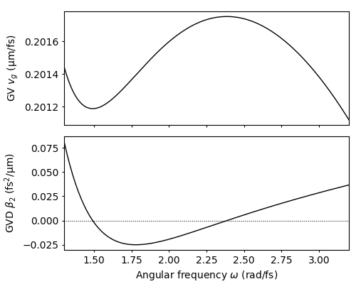
We then visually assess the group-velocity (GV) and group-velocity dispersion (GVD) of the propagation constant in the angular frequency range \(\omega \in [1.2,3.2]~\mathrm{rad/fs}\). GV and GVD are implemented by the class methods vg, and beta2, respectively. To generate a quick plot of both, the GV and GVD, we use the function plot_details_prop_const, which is defined in module tools.

w  = np.linspace(1.3, 3.2, 200)
plot_details_prop_const(w, pc.vg(w), pc.beta2(w))

1.2.3.1. Finding zero-dispersion points

A quick visual assessment of the GVD in the bottom subfigure allows to roughly locate the first zero-dispersion point within the angular frequency interval \([1.4,1.7]~\mathrm{rad/fs}\). The second zero-dispersion point surely falls into the interval \([2.2,2.5]~\mathrm{rad/fs}\). From these rough estimates we can determine the exact roots of \(\beta_2\) as shown below:

w_Z1 = pc.find_root_beta2(1.4, 1.7)
w_Z2 = pc.find_root_beta2(2.2, 2.5)

print('w_Z1 = ', w_Z1)
print('w_Z2 = ', w_Z2)

Out:

w_Z1 =  1.4907331965874615
w_Z2 =  2.385682823499155

1.2.3.2. Finding group-velocity matched frequencies

For the desing of propagation scenarios that demonstrate, e.g., the interaction of a soliton and a dispersive wave accross a zero-dispersion point, it is useful to be able to compute a group-velocity matched partner frequency for a give frequency. Using the PropConst convenience class this can be done as shown below. Consider, e.g., a soliton with center frequency \(\omega_{\rm{S}}=2.1~\mathrm{rad/fs}\). Then, a group-velocity matched frequency in the domain of normal dispersion (for \(\omega>2.386\)), which surely is contained in the interval \(\omega\in[2.4,3.0]\), can be computed as follows:

w_S = 2.1
w_GVM = pc.find_match_beta1(w_S, 2.4, 3.0)

print('w_GVM = ', w_GVM)

Out:

w_GVM =  2.6757196927682507

We might then reassure us that both frequencies exhibit the same group-velocity like so:

print(np.abs(pc.vg(w_S)-pc.vg(w_GVM)) < 1e-6 )

Out:

True

1.2.3.3. Computing local expansion coefficients of \(\beta(\omega)\)

Taylor expansion coefficients of the proapgation constant at a specific frequency can be computed as shown below. Consider, e.g., the frequency \(\omega_{\rm{S}}=2.1~\mathrm{rad/fs}\), located in the domain of anomalous dispersion. The local expansion coefficients of \(\beta\) up to order \(n_{\rm{max}}=6\) at that specific point are obtained by

beta_coeffs = pc.compute_expansion_coefficients(w_S, n_max=5)

for idx, coeff in enumerate(beta_coeffs):
    print("beta_{:d} = {:10.7f} fs^{:d}/micron".format(idx, coeff, idx))

Out:

beta_0 = 10.1264331 fs^0/micron
beta_1 =  4.9586473 fs^1/micron
beta_2 = -0.0073170 fs^2/micron
beta_3 =  0.0081117 fs^3/micron
beta_4 =  0.0017631 fs^4/micron
beta_5 = -0.0030165 fs^5/micron