1.2.5. Using a specific Raman response function

This examples shows how the different Raman response functions, implemented in modeule raman_response, can be used with the class CustomModelPCF (derived from the more generic class FMAS_S_R), implemented in module models.

A side-by-side comparison of the frequency-domain representation of the different Raman response models is detailed under

Implemented Raman response functions

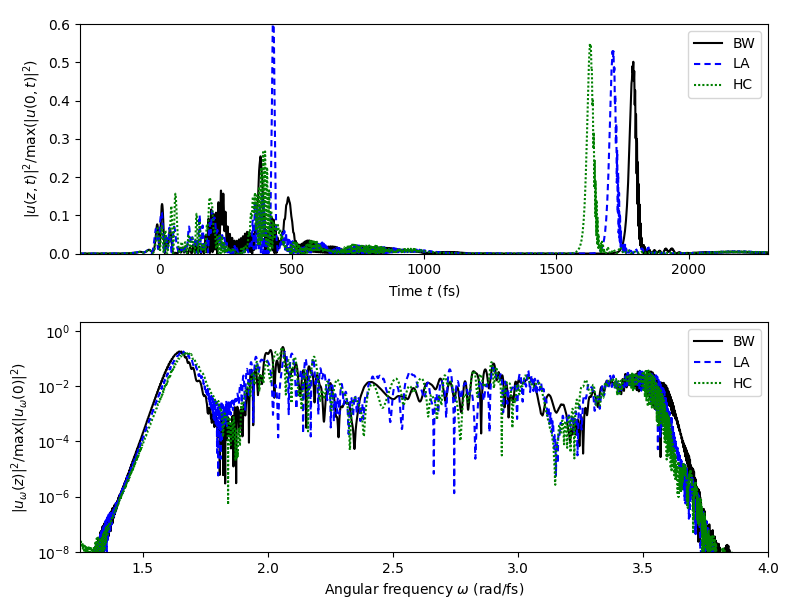
In particular, this example shows how the implemented Raman response models affect the dynamical evolution of the exemplary use case:

Supercontinuum generation in a PCF

We first import the functionality needed to define the problem specific data structures such as the model, we will use the CustomModelPCF defined module models, the computational grid, and the \(z\)-propagation algorithm. The various Raman response models, which we demonstrate here, will be imported later where they are needed in the workflow.

import fmas
import numpy as np
from fmas.models import CustomModelPCF
from fmas.grid import Grid
from fmas.analytic_signal import AS
from fmas.solver import IFM_RK4IP
from fmas.tools import plot_evolution
from fmas.config import FTSHIFT

Since we will perform a sequence of numerical simulations, we first define and initialize all data structures and variables common to the different simulation runs:

# -- COMPUTATIONAL DOMAIN
t_max = 3500.       # (fs)
t_num = 2**14       # (-)
z_max = 0.10*1e6    # (micron)
z_num = 8000        # (-)
z_skip = 10         # (-)

# -- INITIAL CONDITION
P0 = 1e4            # (W)
t0 = 28.4           # (fs)
w0 = 2.2559         # (rad/fs)
E_0t_fun = lambda t: np.real(np.sqrt(P0)/np.cosh(t/t0)*np.exp(-1j*w0*t))

# -- COMPUTATIONAL DOMAIN
grid = Grid( t_max = t_max, t_num = t_num, z_max = z_max, z_num = z_num)
# -- PROPAGATION MODEL
model = CustomModelPCF(w=grid.w)
# -- ANALYTIC SIGNAL INITIAL CONDITION
ic = AS(E_0t_fun(grid.t))

We first perfom a simulation run using the default Raman response model implemented with CustomModelPCF. This is also implemented in terms of the Blow-Wood type response model h_BW in module raman_response. From the simulation results we will only keep the final \(z\)-slice.

# -- INITIALIZE MODEL
solver = IFM_RK4IP( model.Lw, model.Nw, user_action = model.claw)
# -- SET INITIAL CONDITION
solver.set_initial_condition( grid.w, AS(E_0t_fun(grid.t)).w_rep)
# -- z-PROPAGATION
solver.propagate( z_range = z_max, n_steps = z_num, n_skip = z_skip)

# -- KEEP ONLY LAST z-SLICE
ut_BW, uw_BW = solver.utz[-1], solver.uwz[-1]

To use a Raman response function different from the default requires two steps: first, the desired Raman response model needs to be imported from module raman_response (or it has to be defined by the user in any other way); second, the default response function of the model has to be overwritten. Below we show this for two Raman response functions that differ from the default response model of CustomModelPCF.

First, we consider the Lin-Agrawal type Raman response, which is implemented as function h_LA in module raman_response. If a different value for the fractional Raman contribution is needed, the corresponding class attribute can be overwritten as well:

from fmas.raman_response import h_LA

model.hRw = h_LA(grid.t) # overwrite default resonse function
model.fR = 0.18          # overwrite default fractional Raman response if needed

solver = IFM_RK4IP( model.Lw, model.Nw, user_action = model.claw)
solver.set_initial_condition( grid.w, AS(E_0t_fun(grid.t)).w_rep)
solver.propagate( z_range = z_max, n_steps = z_num, n_skip = z_skip)
ut_LA, uw_LA = solver.utz[-1], solver.uwz[-1]

Next, we perform a simulation using the Hollenbeck-Cantrell type Raman response, which is implemented as function h_HC in module raman_response:

from fmas.raman_response import h_HC

model.hRw = h_HC(grid.t)

# -- PERFORM SIMULATION
solver = IFM_RK4IP( model.Lw, model.Nw, user_action = model.claw)
solver.set_initial_condition( grid.w, AS(E_0t_fun(grid.t)).w_rep)
solver.propagate( z_range = z_max, n_steps = z_num, n_skip = z_skip)
ut_HC, uw_HC = solver.utz[-1], solver.uwz[-1]

The subsequent plot compares the effect of three Raman response models side-by-side:

import matplotlib as mpl
import matplotlib.pyplot as plt
import matplotlib.colors as col

# -- INITIAL PEAK INTENSITIES (FOR NORMALIZATION)
It0 = np.max(np.abs(ic.t_rep)**2)
Iw0 = np.max(np.abs(ic.w_rep)**2)

f, (ax1, ax2) = plt.subplots(2, 1, figsize=(8,6))
plt.subplots_adjust(left=0.1, right=0.96, bottom=0.08, top=0.96, wspace=0.3, hspace=0.3)

ax1.plot(grid.t, np.abs(ut_BW)**2/It0, color='k', label=r'BW')
ax1.plot(grid.t, np.abs(ut_LA)**2/It0, color='blue', dashes=[3,2], label=r'LA')
ax1.plot(grid.t, np.abs(ut_HC)**2/It0, color='green', dashes=[1,1], label=r'HC')
ax1.set_yscale('linear')
ax1.set_xlim(-300,2300)
ax1.set_ylim(0.,0.6)
ax1.set_xlabel('Time $t~(\mathrm{fs})$')
ax1.set_ylabel('$|u(z,t)|^2/\max(|u(0,t)|^2)$')
ax1.legend()

ax2.plot(grid.w, np.abs(uw_BW)**2/Iw0, color='k', label=r'BW')
ax2.plot(grid.w, np.abs(uw_LA)**2/Iw0, color='blue', dashes=[3,2], label=r'LA')
ax2.plot(grid.w, np.abs(uw_HC)**2/Iw0, color='green', dashes=[1,1], label=r'HC')
ax2.set_xlim(1.25,4.0)
ax2.set_xlabel('Angular frequency $\omega~(\mathrm{rad/fs})$')
ax2.set_ylim(1e-8,2)
ax2.set_yscale('log')
ax2.set_ylabel('$|u_\omega(z)|^2/\max(|u_\omega(0)|^2)$')
ax2.legend()

plt.show()