1.2.2. Implemented Raman response functions

This examples shows the frequency-domain representation of the different Raman response models, implemented in modeule raman_response.

An example demonstrating how the implemented Raman response models affect the dynamical evolution of a specific propagation scenario is shown under

Using a specific Raman response function

We first import the functionality needed to produce a plot containing all the implemented Raman response models

import numpy as np
from fmas.grid import Grid
from fmas.raman_response import h_BW, h_LA, h_HC

We then set up a data structure providing a discrete time and frequency axes

grid = Grid(
    t_max = 3500., # (fs)
    t_num = 2**14  # (-)
)

Next we initialize the frequency-domain representation of the different Raman response models

hw_BW = h_BW(grid.t)
hw_LA = h_LA(grid.t)
hw_HC = h_HC(grid.t)

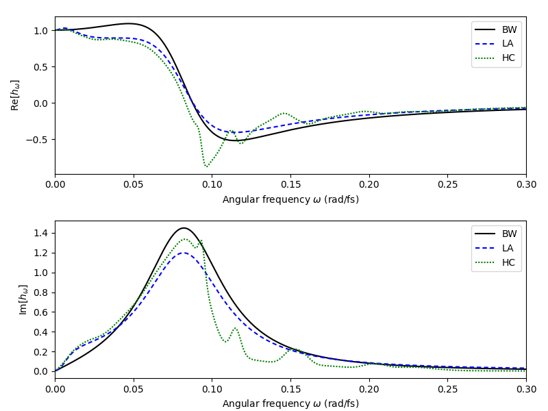
The subsequent plot compares the three Raman response models side-by-side. The subplot on top shows the real part of the frequency-domain representation of the Raman response, the subplot at the bottom shows the respective imaginary parts (i.e. the Raman gain spectrum):

import matplotlib as mpl
import matplotlib.pyplot as plt
import matplotlib.colors as col

w_min, w_max = 0., 0.3
w_mask = np.logical_and(grid.w>w_min, grid.w<w_max)

f, (ax1, ax2) = plt.subplots(2, 1, figsize=(8,6))
plt.subplots_adjust(left=0.1, right=0.96, bottom=0.08, top=0.96, wspace=0.3, hspace=0.3)

ax1.plot(grid.w[w_mask], np.real(hw_BW[w_mask]), color='k', label=r'BW')
ax1.plot(grid.w[w_mask], np.real(hw_LA[w_mask]), color='blue', dashes=[3,2], label=r'LA')
ax1.plot(grid.w[w_mask], np.real(hw_HC[w_mask]), color='green', dashes=[1,1], label=r'HC')
ax1.set_xlim(w_min,w_max)
ax1.set_xlabel('Angular frequency $\omega~(\mathrm{rad/fs})$')
ax1.set_ylabel('$\mathsf{Re}[h_\omega]$')
ax1.legend()

ax2.plot(grid.w[w_mask], np.imag(hw_BW[w_mask]), color='k', label=r'BW')
ax2.plot(grid.w[w_mask], np.imag(hw_LA[w_mask]), color='blue', dashes=[3,2], label=r'LA')
ax2.plot(grid.w[w_mask], np.imag(hw_HC[w_mask]), color='green', dashes=[1,1], label=r'HC')
ax2.set_xlim(w_min,w_max)
ax2.set_xlabel('Angular frequency $\omega~(\mathrm{rad/fs})$')
ax2.set_ylabel('$\mathsf{Im}[h_\omega]$')
ax2.legend()

plt.show()