1.2.6. Implementing a custom model

This examples shows how to use the \(z\)-propagation model FMAS_S_Raman to implement a specialized propagation model, using a cutom propagation constant and custom parameters for the Raman response function.

import fmas
import numpy as np
from fmas.models import FMAS_S_Raman
from fmas.solver import IFM_RK4IP
from fmas.analytic_signal import AS
from fmas.grid import Grid
from fmas.tools import plot_spectrogram, spectrogram
from fmas.propagation_constant import PropConst
from fmas.tools import sech, plot_details_prop_const
from fmas.tools import change_reference_frame, plot_evolution

Below we will demonstrate how to implement a specialized \(z\)-propagation model with propagation constant of a ZBLAN fiber [1], and a Raman response function with parameters suited for simulating such a fiber [2]. Specifically, we here reproduce the ZBLAN model of Ref. [3].

This example shows that, while the implemented class FMAS_S_Raman can be used with custom paramters, it can also serve as a superclass for a specialized model.

We first start by deriving a subclass from FMAS_S_Raman, equipped with the desired properties

class ZBLAN(FMAS_S_Raman):
    r"""Custom model for ZBLAN fiber.

    Implements the :math:`z`-propagation model for a ZBLAN fiber, using the
    proapagation constant and Raman response function parameters of Ref. [1].
    Parameters that specify the Raman response function and `n_2` are taken
    from Ref. [2].

    References:
        [1] A. Demircan, Sh. Amiranashvili, C. Bree, U. Morgner, G. Steinmeyer,
        Adjustable pulse compression scheme for generation of few-cycle pulses
        in the midinfrared, Opt. Lett. 39 (2014) 2735,
        https://doi.org/10.1364/OL.39.002735.

        [2] L. Liu, G. Qin, Q. Tian, D. Zhao, W. Qin, Numerical investigation
        of mid-infrared supercontinuum generation up to 5 μm in single mode
        fluoride fiber, Opt. Exp. 19 (2011) 10041,
        https://doi.org/10.1364/OE.19.010041.

    Args:
        w (:obj:`numpy.ndarray`): Angular frequency grid.

    Returns:
        :obj:`numpy.ndarray` Propagation constant as function of
        frequency detuning.
    """
    def __init__(self, w, fR=0.1929, tau1=9.0, tau2=134.0):

        # -- SPECIFY MODEL SPECIFIC PARAMETERS
        n2 = 2.1e-2     # (micron^2/W)

        # -- LOCAL HELPER FUNCTION FOR PROPAGATION CONSTANT
        def _define_beta_fun_ZBLAN():
            r"""Custom propagation constant for ZBLAN fiber.

            Implements rational Pade-approximant of order [4/4] for the
            refractive index of a ZBLAN fiber (PCF).

            Returns:
                :obj:`callable`: Propagation constant for NL-PM-750 PCF.
            """
            p = np.poly1d((11.3882,0.,760.771,0.,-1.)[::-1])
            q = np.poly1d(( 8.69689, 0.,351.039,0.,-1.)[::-1])
            n_idx = lambda w: np.sqrt(p(w)/q(w))     # (-)
            b2Roots = (0.25816960569391839,1.1756233558942193)
            c0 = 0.29979                    # (micron/fs)
            return lambda w: n_idx(w)*w/c0  # (1/micron)

        # -- MAKE PROPAGATION CONSTANT A CLASS ATTRIBUTE
        self.beta_fun = _define_beta_fun_ZBLAN()
        # -- EQUIP THE SUPERCLASS
        super().__init__(w, self.beta_fun(w), n2, fR, tau1, tau2)

Next, we use the implemente class to reproduce the interaction between a soliton and a dispersive wave in absence of the Raman effect. In particular, we here reproduce the collision scenario underlying Fig. 2 of Ref. [3].

Therefore, we initialize an adequate computational domain and an instance of the ZBLAN model, for which the fractional contribution of the Raman effect is set to zero

grid = Grid(
    t_max = 4500.,       # (fs)
    t_num = 2**14        # (-)
)

model = ZBLAN(grid.w, fR=0.0)

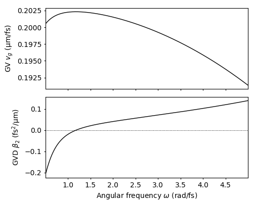
To visually assess the group-velocity (GV) and group-velocity dispersion (GVD) of the propagation constant in the relevant angular frequency range we use the convenience class PropConst and pre-implemented plotting functions that are implemented in module tools

w = grid.w[np.logical_and(grid.w>0.5,grid.w<5.)]
pc = PropConst(model.beta_fun)
plot_details_prop_const(w, pc.vg(w), pc.beta2(w))

Next, we prepare the corresponding initial condition, which is well described in Ref. [3]. It consists of a fundamental soliton with duration \(t_{\rm{S}}=25.2\,\mathrm{fs}\) and center frequency \(\omega_{\rm{S}}=0.4709\,\mathrm{rad/fs}\), and a dispersive wave with duration \(t_{\rm{DW}}=100\,\mathrm{fs}\) and angular frequency \(\omega_{\rm{DW}}=2.6177\,\mathrm{rad/fs}\). Both pulses exhibit an amplitude ratio of \(A_{\rm{DW}}/A_{\rm{S}}=0.566\), and the soliton is launched with deltay \(t_{\rm{off}}=450\,\mathrm{fs}\).

wS, tS = 0.4709, 25.2   # (rad/fs), (fs)
wDW, tDW = 2.6177, 100. # (rad/fs), (fs)
t_off = -450.           # (fs)
rDW = 0.566             # (-)
A0S = np.sqrt(abs(pc.beta2(wS))*model.c0/wS/model.n2)/tS
E_0t = np.real(
            A0S*sech(grid.t/tS)*np.exp(1j*wS*grid.t) +               # S
            rDW*A0S*sech((grid.t-t_off)/tDW)*np.exp(1j*wDW*grid.t) ) # DW
Eps_0w =  AS(E_0t).w_rep

For \(z\)-propagation we here use a variant of an integrating factor method, referred to as the “Runge-Kutta in the interaction picture” method, implemented as IFM_RK4IP in module solver.

solver = IFM_RK4IP( model.Lw, model.Nw)
solver.set_initial_condition( grid.w,Eps_0w)

solver.propagate(
    z_range = 0.35e6,   # (micron)
    n_steps = 4000,     # (-)
    n_skip = 10         # (-)
)

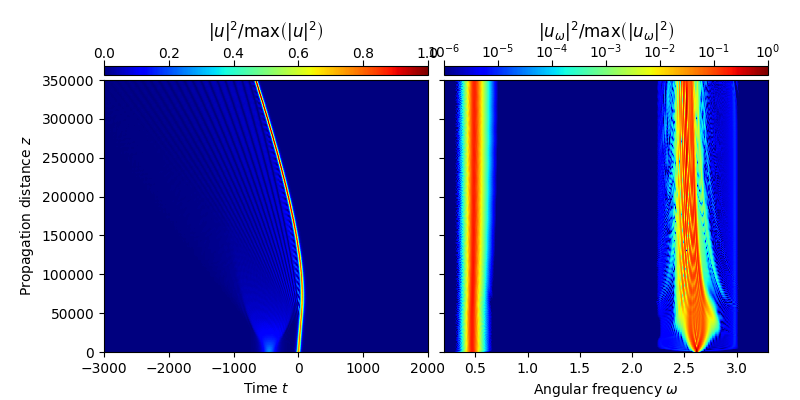
Finally, the \(z\)-propagation characteristics of the interaction process can be obtained by

utz = change_reference_frame(solver.w, solver.z, solver.uwz, pc.vg(wS))
plot_evolution( solver.z, grid.t, utz, t_lim=(-3000,2000), w_lim=(0.2,3.3))

# sphinx_gallery_thumbnail_number = 2

References:

[1] C. Agger, C. Petersen, S. Dupont, H. Steffensen, J. K. Lyngso, C. L. Thomsen, J. Thogersen, S. R. Keiding, O. Bang, Supercontinuum generation in ZBLAN fibers—detailed comparison between measurement and simulation, J. Opt. Soc. Am. B 29 (2012) 635, https://doi.org/10.1364/JOSAB.29.000635.

[2] L. Liu, G. Qin, Q. Tian, D. Zhao, W. Qin, Numerical investigation of mid-infrared supercontinuum generation up to 5 μm in single mode fluoride fiber, Opt. Exp. 19 (2011) 10041, https://doi.org/10.1364/OE.19.010041.

[3] A. Demircan, Sh. Amiranashvili, C. Bree, U. Morgner, G. Steinmeyer, Adjustable pulse compression scheme for generation of few-cycle pulses in the midinfrared, Opt. Lett. 39 (2014) 2735, https://doi.org/10.1364/OL.39.002735.