2.1.3. Extending py-fmas by optfrog spectrograms

This examples shows how to use the py-fmas library code in conjunction with the optFrog spectrogram tool.

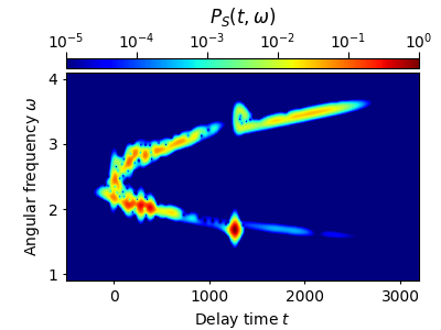
In particular, the example details a numerical experiment performing pulse propagation in terms of the simplified forward model for the analytic signal including the Raman effect [1]. Here, the model is used to perform simulations on supercontinuum generation for an instance of a highly nonlinear photonic crystal fiber (PCF) with an anomalous group-velocity dispersion regime [2]. The example also includes data postprocessing by calculating an analytic signal spectrum with optimized time-frequency resolution using the optfrog-tool [3].

An example that shows how to use the simple py-fmas native spectrogram is shown under the link below:

Computing spectrograms

Note:

• For this exampe to run, the optfrog tool needs to be installed [3].

• The py-fmas package includes a simple spectrogram in module tools. The optfrog Python package however includes extended functionality by allowing a user to calculate spectrograms with optimized time and frequency resolution.

References:

[1] A. Demircan, Sh. Amiranashvili, C. Bree, C. Mahnke, F. Mitschke, G. Steinmeyer, Rogue wave formation by accelerated solitons at an optical event horizon, Appl. Phys. B 115 (2014) 343, http://dx.doi.org/10.1007/s00340-013-5609-9

[2] J. M. Dudley, G. Genty, S. Coen, Supercontinuum generation in photonic crystal fiber, Rev. Mod. Phys. 78 (2006) 1135, http://dx.doi.org/10.1103/RevModPhys.78.1135

[3] O. Melchert, B. Roth, U. Morgner, A. Demircan, OptFROG — Analytic signal spectrograms with optimized time–frequency resolution, SoftwareX 10 (2019) 100275, https://doi.org/10.1016/j.softx.2019.100275, code repository: https://github.com/ElsevierSoftwareX/SOFTX_2019_130.

Out:

# optFrog convergence info:
# (sigma) (Q(sigma, alpha=0.000000)) (IAE1) (IAE2)
355.959086 0.570680 1.101932 0.039428
573.313374 0.616589 1.200919 0.032259
221.626749 0.531656 0.991327 0.071986
138.604799 0.507169 0.892059 0.122278
87.294411 0.488869 0.786706 0.191033
55.582848 0.466704 0.665983 0.267425
35.984024 0.447466 0.541951 0.352981
23.871285 0.437389 0.432716 0.442062
16.385200 0.445184 0.354833 0.535534
25.575392 0.438465 0.449987 0.426944
22.988308 0.437094 0.423509 0.450678
20.466145 0.438235 0.397714 0.478756
22.706287 0.437021 0.420520 0.453522
21.850629 0.437280 0.411743 0.462818
22.585945 0.437029 0.419271 0.454787
22.688130 0.437019 0.420330 0.453708
22.665447 0.437019 0.420096 0.453943
22.679466 0.437019 0.420241 0.453797
22.677702 0.437019 0.420223 0.453815
22.673021 0.437019 0.420174 0.453863
22.674907 0.437018 0.420194 0.453843
22.675229 0.437018 0.420197 0.453840
22.674560 0.437018 0.420190 0.453847
22.673972 0.437018 0.420184 0.453853
22.674336 0.437018 0.420188 0.453849
22.674510 0.437018 0.420190 0.453847
22.674467 0.437018 0.420189 0.453848
22.674417 0.437018 0.420189 0.453848
22.674443 0.437018 0.420189 0.453848
22.674439 0.437018 0.420189 0.453848
22.674431 0.437018 0.420189 0.453848
22.674436 0.437018 0.420189 0.453848

import fmas
import numpy as np
from fmas.models import CustomModelPCF
from fmas.solver import IFM_RK4IP
from fmas.analytic_signal import AS
from fmas.grid import Grid
from fmas.tools import plot_spectrogram
from optfrog import optFrog


def main():
    # -- DEFINE SIMULATION PARAMETERS
    # ... COMPUTATIONAL DOMAIN
    t_max = 3500.       # (fs)
    t_num = 2**14       # (-)
    z_max = 0.10*1e6    # (micron)
    z_num = 8000        # (-)
    z_skip = 10         # (-)
    # ... INITIAL CONDITION
    P0 = 1e4            # (W)
    t0 = 28.4           # (fs)
    w0 = 2.2559         # (rad/fs)
    E_0t_fun = lambda t: np.real(np.sqrt(P0)/np.cosh(t/t0)*np.exp(-1j*w0*t))

    # -- INITIALIZATION STAGE
    grid = Grid( t_max = t_max, t_num = t_num, z_max = z_max, z_num = z_num)
    model = CustomModelPCF(w=grid.w)
    solver = IFM_RK4IP( model.Lw, model.Nw, user_action = model.claw)
    solver.set_initial_condition( grid.w, AS(E_0t_fun(grid.t)).w_rep)
    # -- RUN SIMULATION
    solver.propagate( z_range = z_max, n_steps = z_num, n_skip = z_skip)

    # -- POSTPRICESSING: COMPUTE SPECTROGRAM USING OPTFROG
    # ... Z-DISTANCE, Z-INDEX AND FIELD FOR WHICH TO COMPUTE TRACE
    z0 = 0.08e6  # (micron)
    z0_idx = np.argmin(np.abs(solver.z-z0))
    Et = solver.utz[z0_idx]
    # ... WINDOW FUNCTION FOR SIGNAL LOCALIZATION
    def window_fun(s0):
        return lambda t: np.exp(-t**2/2/s0/s0)/np.sqrt(2.*np.pi)/s0
    # ... OPTFROG TRACE
    res = optFrog(
        grid.t,                         # TEMPORAL GRID
        Et,                             # ANALYTIC SIGNAL
        window_fun,                     # WINDOW FUNCTION
        tLim = (-500.0, 3200.0, 10),    # (tmin, fs) (tmax, fs) (nskip)
        wLim = (0.9, 4.1, 3)            # (wmin, fs) (wmax, fs) (nskip)
    )
    # ... SHOW SPECTROGRAM
    plot_spectrogram(res.tau, res.w, res.P)


if __name__=='__main__':
    main()