2.1.5. Four pulse interaction in a ESM PCF

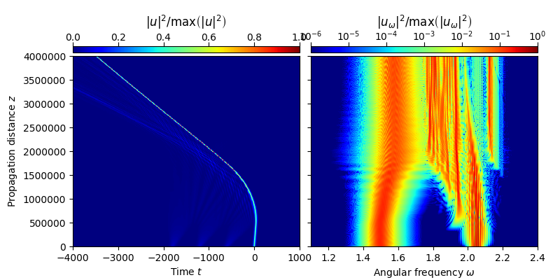
This examples demonstrates the interaction between a fundamental soliton and a three dispersive wave with pairwise distinct center frequencies in an “endlessly single mode” (ESM) photonic crystal fiber. For the numerical simualtion the simplified forward model for the analytic signal is used [3].

References:

[1] A. Demircan, Sh. Amiranashvili, C. Bree, C. Mahnke, F. Mitschke, G. Steinmeyer, Rogue wave formation by accelerated solitons at an optical event horizon, Appl. Phys. B 115 (2014) 343, http://dx.doi.org/10.1007/s00340-013-5609-9

import fmas
import numpy as np
from fmas.grid import Grid
from fmas.models import FMAS_S
from fmas.solver import IFM_RK4IP
from fmas.analytic_signal import AS
from fmas.tools import change_reference_frame, plot_evolution
from fmas.propagation_constant import PropConst


def define_beta_fun_ESM():
    r"""Custom propagation constant for an ESM photonic crystal fiber.

    Implements rational Pade-approximant of order [8/8] for the refractive
    index of a endlessly single mode (ESM) nonlinear photonic crystal fiber
    (PCF), see Ref. [1].

    References:
        [1] Visibly 'white' light generation in uniform photonic crystal fiber
        using a microchip laser Stone, J.M. and Knight, J.C.  Optics Express 16
        (2007) 2670.

    Returns:
        :obj:`callable`: Propagation constant for ESM PCF.
    """
    p = np.poly1d(
        (16.89475, 0., -319.13216, 0., 34.82210, 0., -0.992495, 0., 0.0010671)[::-1])
    q = np.poly1d(
        ( 1.00000, 0., -702.70157, 0., 78.28249, 0., -2.337086, 0., 0.0062267)[::-1])
    n_idx = lambda w: 1+p(w)/q(w) # (-)
    c0 = 0.29979                    # (micron/fs)
    return lambda w: n_idx(w)*w/c0   # (1/micron)


def main():

    # -- DEFINE SIMULATION PARAMETERS
    # ... COMPUTATIONAL DOMAIN
    t_max = 4000.       # (fs)
    t_num = 2**14       # (-)
    z_max = 4.0e6       # (micron)
    z_num = 50000       # (-)
    z_skip =100         # (-)
    n2 = 3.0e-8         # (micron^2/W)

    beta_fun = define_beta_fun_ESM()
    pc = PropConst(beta_fun)

    # -- INITIALIZATION STAGE
    grid = Grid( t_max = t_max, t_num = t_num, z_max = z_max, z_num = z_num)
    model = FMAS_S(w=grid.w, beta_w=pc.beta(grid.w), n2=n2)
    solver = IFM_RK4IP( model.Lw, model.Nw, user_action = model.claw)

    # -- SET UP INITIAL CONDITION
    t = grid.t
    # ... FUNDAMENTAL NSE SOLITON
    w0_S, t0_S = 1.5, 20.   # (rad/fs), (fs)
    A0 = np.sqrt(abs(pc.beta2(w0_S))*model.c0/w0_S/n2)/t0_S
    A0_S = A0/np.cosh(t/t0_S)*np.exp(1j*w0_S*t)
    # ... 1ST DISPERSIVE WAVE; UNITS (rad/fs), (fs), (fs), (-)
    w0_DW1, t0_DW1, t_off1, s1 = 2.06, 60., -600., 0.35
    A0_DW1 = s1*A0/np.cosh((t-t_off1)/t0_DW1)*np.exp(1j*w0_DW1*t)
    # ... 2ND DISPERSIVE WAVE; UNITS (rad/fs), (fs), (fs), (-)
    w0_DW2, t0_DW2, t_off2, s2 = 2.05, 60., -1200., 0.35
    A0_DW2 = s2*A0/np.cosh((t-t_off2)/t0_DW2)*np.exp(1j*w0_DW2*t)
    # ... 3RD DISPERSIVE WAVE; UNITS (rad/fs), (fs), (fs), (-)
    w0_DW3, t0_DW3, t_off3, s3 = 2.04, 60., -1800., 0.35
    A0_DW3 = s3*A0/np.cosh((t-t_off3)/t0_DW3)*np.exp(1j*w0_DW3*t)
    # ... ANALYTIC SIGNAL OF FULL ININITIAL CONDITION
    Eps_0w = AS(np.real(A0_S + A0_DW1 + A0_DW2 + A0_DW3)).w_rep

    solver.set_initial_condition( grid.w, Eps_0w)
    solver.propagate( z_range = z_max, n_steps = z_num, n_skip = z_skip)

    # -- SHOW RESULTS
    v0 = pc.vg(w0_S)
    utz = change_reference_frame(solver.w, solver.z, solver.uwz, v0)
    plot_evolution( solver.z, grid.t, utz, t_lim=(-4000,1000), w_lim=(1.1,2.4))


if __name__=='__main__':
    main()