2.2.1. Superimposed fundamental solitons

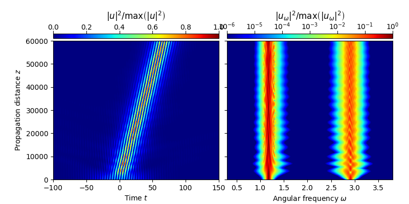
This examples demonstrates the generation of two-frequency soliton molecules, using the forward model for the analytic signal [1,2], in py-fmas implemented as FMAS.

In particular, this example shows how soliton molecules are generated from two initially superimposed fundamental solitons at distinctly different frequencies [3]. The exmample reproduces the propagation scenario shown in Fig. S10 of the supplementary material to [3].

References:

[1] Sh. Amiranashvili, A. Demircan, Hamiltonian structure of propagation equations for ultrashort optical pulses, Phys. Rev. E 10 (2010) 013812, http://dx.doi.org/10.1103/PhysRevA.82.013812.

[2] Sh. Amiranashvili, A. Demircan, Ultrashort Optical Pulse Propagation in terms of Analytic Signal, Adv. Opt. Tech. 2011 (2011) 989515, http://dx.doi.org/10.1155/2011/989515.

[3] O. Melchert, S. Willms, S. Bose, A. Yulin, B. Roth, F. Mitschke, U. Morgner, I. Babushkin, A. Demircan, Soliton Molecules with Two Frequencies, Phys. Rev. Lett. 123 (2019) 243905, https://doi.org/10.1103/PhysRevLett.123.243905.

import fmas
import numpy as np
from fmas.grid import Grid
from fmas.models import FMAS
from fmas.solver import IFM_RK4IP
from fmas.analytic_signal import AS
from fmas.tools import change_reference_frame, plot_evolution
from fmas.propagation_constant import PropConst


def define_beta_fun():
    r"""Custom refractive index.
    """
    p = np.poly1d((9.653881, -39.738626, 16.8848987, -2.745456)[::-1])
    q = np.poly1d((1.000000,  -9.496406,  4.2206250, -0.703437)[::-1])
    n_idx = lambda w: p(w)/q(w)     # (-)
    c0 = 0.29979                    # (micron/fs)
    return lambda w: n_idx(w)*w/c0  # (1/micron)

def main():

    t_max = 2000.           # (fs)
    t_num = 2**14           # (-)
    z_max =  0.06e6         # (micron)
    z_num = 25000           # (-)
    z_skip = 50             # (-)
    chi = 1.0               # (micron^2/W)
    c0 = 0.29979            # (micron/fs)

    # -- PROPAGATION CONSTANT
    beta_fun = define_beta_fun()
    pc = PropConst(beta_fun)

    # -- INITIALIZE DATA-STRUCTURES AND ALGORITHMS
    grid = Grid( t_max = t_max, t_num = t_num, z_max = z_max, z_num = z_num)
    model = FMAS(w=grid.w, beta_w = beta_fun(grid.w), chi = chi )
    solver = IFM_RK4IP( model.Lw, model.Nw, user_action = model.claw)

    # -- PREPARE INITIAL CONDITION AND RUN SIMULATION
    w01, t01, A01 = 1.178, 30.0,  0.0248892 # (rad/fs), (fs), (sqrt(W))
    w02, t02, A02 = 2.909, 30.0, 0.0136676  # (rad/fs), (fs), (sqrt(W))
    A_0t_fun = lambda t, A0, t0, w0: np.real(A0/np.cosh(t/t0)*np.exp(1j*w0*t))
    E_0t = A_0t_fun(grid.t, A01, t01, w01) + A_0t_fun(grid.t, A02, t02, w02)
    solver.set_initial_condition( grid.w, AS(E_0t).w_rep)
    solver.propagate( z_range = z_max, n_steps = z_num, n_skip = z_skip)

    # -- SHOW RESULTS IN MOVING FRAME OF REFERENCE
    v0 = 0.0749641870819 # (micron/fs)
    utz = change_reference_frame(solver.w, solver.z, solver.uwz, v0)
    plot_evolution( solver.z, grid.t, utz, t_lim=(-100,150), w_lim=(0.3,3.8))


if __name__=='__main__':
    main()