2.2.2. Soliton-soliton collision

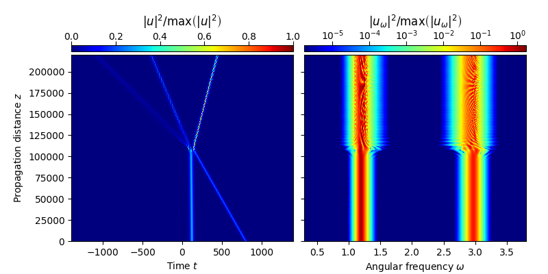
This examples demonstrates the generation of two-frequency soliton molecules, using the forward model for the analytic signal [1,2], in py-fmas implemented as FMAS.

In particular, this example shows how soliton molecules are generated from the collison of two initially well separated fundamental solitons at distinctly different frequencies [3]. The exmample reproduces the propagation scenario shown in Fig. S11 of the supplementary material to [3].

In this example also some pre-processing of the solitons is done to reduce the amount of excess radtion in the computational domain.

References:

[1] Sh. Amiranashvili, A. Demircan, Hamiltonian structure of propagation equations for ultrashort optical pulses, Phys. Rev. E 10 (2010) 013812, http://dx.doi.org/10.1103/PhysRevA.82.013812.

[2] Sh. Amiranashvili, A. Demircan, Ultrashort Optical Pulse Propagation in terms of Analytic Signal, Adv. Opt. Tech. 2011 (2011) 989515, http://dx.doi.org/10.1155/2011/989515.

[3] O. Melchert, S. Willms, S. Bose, A. Yulin, B. Roth, F. Mitschke, U. Morgner, I. Babushkin, A. Demircan, Soliton Molecules with Two Frequencies, Phys. Rev. Lett. 123 (2019) 243905, https://doi.org/10.1103/PhysRevLett.123.243905.

import fmas
import numpy as np
from fmas.models import FMAS
from fmas.solver import IFM_RK4IP
from fmas.analytic_signal import AS
from fmas.grid import Grid
from fmas.tools import change_reference_frame, plot_evolution
from fmas.propagation_constant import PropConst


def define_beta_fun():
    r"""Custom refractive index.
    """
    p = np.poly1d((9.653881, -39.738626, 16.8848987, -2.745456)[::-1])
    q = np.poly1d((1.000000,  -9.496406,  4.2206250, -0.703437)[::-1])
    n_idx = lambda w: p(w)/q(w)     # (-)
    c0 = 0.29979                    # (micron/fs)
    return lambda w: n_idx(w)*w/c0  # (1/micron)


def main():

    t_max = 2000.           # (fs)
    t_num = 2**14           # (-)
    chi = 1.0               # (micron^2/W)
    c0 = 0.29979            # (micron/fs)

    # -- PROPAGATION CONSTANT
    beta_fun = define_beta_fun()
    pc = PropConst(beta_fun)

    grid = Grid( t_max = t_max, t_num = t_num)
    model = FMAS(w=grid.w, beta_w = beta_fun(grid.w), chi = chi )
    solver = IFM_RK4IP( model.Lw, model.Nw, user_action = model.claw)

    # -- FUNDAMENTAL SOLITON INTITIAL CONDITION
    A_0t_fun = lambda t, A0, t0, w0: np.real(A0/np.cosh(t/t0)*np.exp(1j*w0*t))
    # ... FIRST SOLITON: PROPAGATE AND CLEAN-UP PRIOR TO COLLISION
    w01, t01, A01 = 1.2, 20.0,  0.0351187       # (rad/fs), (fs), (sqrt(W))
    z_max, z_num, z_skip = 0.06e6, 6000, 200    # (micron), (-), (-)
    A_0t_1 = A_0t_fun(grid.t, A01, t01, w01)
    solver.set_initial_condition( grid.w, AS(A_0t_1).w_rep)
    solver.propagate( z_range = z_max, n_steps = z_num, n_skip = z_skip)
    A_0t_1_f = np.real(
                 np.where(
                    np.logical_and(grid.t>-15., grid.t<273.0),
                    solver.utz[-1],
                    0j
                 )
               )
    solver.clear()

    # ... SECOND SOLITON: PROPAGATE AND CLEAN-UP PRIOR TO COLLISION
    w02, t02, A02 = 2.96750, 15.0, 0.0289073    # (rad/fs), (fs), (sqrt(W))
    z_max, z_num, z_skip = 0.06e6, 6000, 200    # (micron), (-), (-)
    A_0t_2 = A_0t_fun(grid.t-800., A02, t02, w02)
    solver.set_initial_condition( grid.w, AS(A_0t_2).w_rep)
    solver.propagate( z_range = z_max, n_steps = z_num, n_skip = z_skip)
    A_0t_2_f = np.real(
                 np.where(
                    np.logical_and(grid.t>435.0, grid.t<727.0),
                    solver.utz[-1],
                    0j
                 )
               )
    solver.clear()

    # -- LET CLEANED-UP SOLITONS COLLIDE
    z_max, z_num, z_skip = 0.22e6, 50000, 100   # (micron), (-), (-)
    solver.set_initial_condition( grid.w, AS( A_0t_1_f + A_0t_2 ).w_rep)
    solver.propagate( z_range = z_max, n_steps = z_num, n_skip = z_skip)

    # -- SHOW RESULTS IN MOVING FRAME OF REFERENCE
    v0 = 0.0749879876745 # (micron/fs)
    utz = change_reference_frame(solver.w, solver.z, solver.uwz, v0)
    plot_evolution( solver.z, grid.t, utz,
        t_lim = (-1400,1400), w_lim = (0.3,3.8), DO_T_LOG=False)


if __name__=='__main__':
    main()