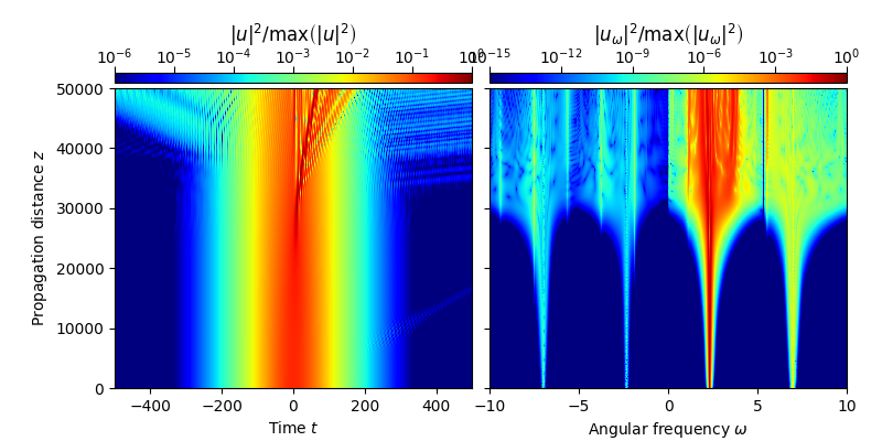
2.3.1. BMCF – Backscattered optical field components

This examples demonstrates backscattered optical field components using the bidirectional model for the complex field (BMCF), described in Ref. [1].

In particular, this example reproduces the propagation scenario shown in Fig. 1(a) of Ref. [1]. The figure shows the evolution of a soliton of duration \(t_{\rm{S}}=50\,\mathrm{fs}\), center frequency \(\omega_{\rm{S}}=2.23548\,\mathrm{rad/fs}\), and soliton order \(N_{\rm{S}}=3.54\). For a detailed discussion, see Ref. [1].

References:

[1] Sh. Amiranashvili, A. Demircan, Hamiltonian structure of propagation equations for ultrashort optical pulses, Phys. Rev. E 10 (2010) 013812, http://dx.doi.org/10.1103/PhysRevA.82.013812.

import fmas
import numpy as np
from fmas.grid import Grid
from fmas.models import BMCF
from fmas.solver import IFM_RK4IP
from fmas.analytic_signal import AS
from fmas.propagation_constant import PropConst, define_beta_fun_fluoride_glass_AD2010
from fmas.tools import change_reference_frame, plot_evolution


def main():

    # -- INITIALIZATION STAGE
    # ... DEFINE SIMULATION PARAMETERS
    t_max = 3500./2     # (fs)
    t_num = 2**14       # (-)
    z_max = 50.0e3      # (micron)
    z_num = 100000      # (-)
    z_skip = 100        # (-)
    c0 = 0.29979        # (micron/fs)
    n2 = 1.             # (micron^2/W) FICTITIOUS VALUE ONLY
    wS = 2.32548        # (rad/fs)
    tS = 50.0           # (fs)
    NS = 3.54           # (-)
    # ... PROPAGGATION CONSTANT
    beta_fun = define_beta_fun_fluoride_glass_AD2010()
    pc = PropConst(beta_fun)
    chi = (8./3)*pc.beta(wS)*c0/wS*n2

    # ... COMPUTATIONAL DOMAIN, MODEL, AND SOLVER
    grid = Grid( t_max = t_max, t_num = t_num, z_max = z_max, z_num = z_num)
    model = BMCF(w=grid.w, beta_w=pc.beta(grid.w), chi =  chi)
    solver = IFM_RK4IP( model.Lw, model.Nw)

    # -- SET UP INITIAL CONDITION
    LD = tS*tS/np.abs( pc.beta2(wS) )
    A0 = NS*np.sqrt(8*c0/wS/n2/LD)
    Eps_0w = AS(np.real(A0/np.cosh(grid.t/tS)*np.exp(1j*wS*grid.t))).w_rep
    solver.set_initial_condition( grid.w, Eps_0w)

    # -- PERFORM Z-PROPAGATION
    solver.propagate( z_range = z_max, n_steps = z_num, n_skip = z_skip)

    # -- SHOW RESULTS
    utz = change_reference_frame(solver.w, solver.z, solver.uwz, pc.vg(wS))
    plot_evolution( solver.z, grid.t, utz,
        t_lim = (-500,500), w_lim = (-10.,10.), DO_T_LOG = True, ratio_Iw=1e-15)


if __name__=='__main__':
    main()