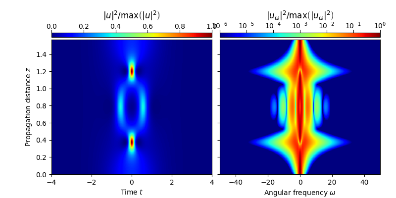
2.3.2. Nonlinear Schrödinger equation – Third-order soliton

This example solves the standard nonlinear Schrödinger equation, given by

\[\partial_z u = -i \frac{\beta_2}{2}\partial_t^2 u + i\gamma |u|^2 u,\]

wherein \(u = u(z, t)\) represents the slowly varying pulse envelope, \(\beta_2=-1\) is the second order dispersion parameter, and \(\gamma=1\) is the nonlinear parameter. As initial condition, a higher-order soliton

\[u_0(t) = N_{\rm{sol}} \sqrt{\frac{|\beta_2|}{\gamma \, t_0^2}} {\rm{sech}}(t/t_0),\]

of duration \(t_0=1\), and soliton order \(N_{\rm{sol}}=3\) is considered. The propagation is performed up to \(z_{\rm{max}}=\pi/2\), i.e. for one soliton period.

import fmas
import numpy as np
from fmas.models import ModelBaseClass
from fmas.config import FTFREQ, FT, IFT, C0
from fmas.solver import SySSM
from fmas.grid import Grid
from fmas.tools import plot_evolution


class NSE(ModelBaseClass):
    def __init__(self, w, b2 = -1.0, gamma = 1.0):
        super().__init__(w, 0.5*b2*w*w)
        self.gamma = gamma

    @property
    def Lw(self):
        return 1j*self.beta_w

    def Nw(self, uw):
        ut = IFT(uw)
        return 1j*self.gamma*FT(np.abs(ut)**2*ut)

    def claw(self, i, zi, w, uw):
        return np.sum(np.abs(uw)**2)


def main():
    # -- DEFINE SIMULATION PARAMETERS
    # ... WAVEGUIDE PROPERTIES
    b2 = -1.0
    gamma = 1.
    # ... TEST PULSE PROPERTIES
    t0 = 1.                       # soliton duration
    P0 = np.abs(b2)/t0/t0/gamma   # peak-intensity
    LD = t0*t0/np.abs(b2)         # dispersion length
    N_sol = 3                     # soliton order
    # ... COMPUTATIONAL DOMAIN
    t_max = 30.
    t_num = 2**12
    z_max  = 0.5*np.pi*LD
    z_num  = 1000
    z_skip = 2

    # -- INITIALIZATION STAGE
    # ... COMPUTATIONAL DOMAIN
    grid = Grid( t_max = t_max, t_num = t_num, z_max = z_max, z_num = z_num)
    # ... NSE MODEL
    model = NSE(grid.w, b2, gamma)
    # ... Z-PROPAGATION USING SYMMETRIC SPLIT-STEP FOURIER METHOD
    solver = SySSM(model.Lw, model.Nw)
    # ... INITIAL CONDITION
    u_0t = N_sol*np.sqrt(P0)/np.cosh(grid.t/t0)
    solver.set_initial_condition(grid.w, FT(u_0t))

    # -- RUN SIMULATION
    solver.propagate(z_range = z_max, n_steps = z_num, n_skip = z_skip)

    plot_evolution( solver.z, grid.t, solver.utz,
        t_lim = (-4,4), w_lim = (-50,50), DO_T_LOG=False)


if __name__=='__main__':
    main()