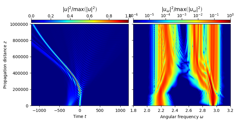
2.1.4. Two pulse interaction in a NLPM750 PCF

This examples demonstrates the interaction between a fundamental soliton and a dispersive wave in a NL-PM-750 photonic crystal fiber. For the numerical simualtion the forward model for the analytic signal including the Raman effect is used [3].

In particular, this example reproduces the propagation scenario for \(t_0=250\,\mathrm{fs}\), shown in Fig.~2(b) of Ref. [2]. Note that here we use a polynomial expansion of the propagation constant, obtained for the reference frequency \(\omega_{\rm{ref}}=1.85\,\mathrm{rad/fs}\). For a more detailed discussion, see Ref. [2].

References:

[1] A. Demircan, Sh. Amiranashvili, C. Bree, C. Mahnke, F. Mitschke, G. Steinmeyer, Rogue wave formation by accelerated solitons at an optical event horizon, Appl. Phys. B 115 (2014) 343, http://dx.doi.org/10.1007/s00340-013-5609-9

[2] O. Melchert, C. Bree, A. Tajalli, A. Pape, R. Arkhipov, S. Willms, I. Babushkin, D. Skryabin, G. Steinmeyer, U. Morgner, A. Demircan, All-optical supercontinuum switching, Communications Physics 3 (2020) 146, https://doi.org/10.1038/s42005-020-00414-1.

import fmas
import numpy as np
from fmas.grid import Grid
from fmas.models import FMAS_S_R
from fmas.solver import IFM_RK4IP
from fmas.analytic_signal import AS
from fmas.propagation_constant import PropConst
from fmas.tools import change_reference_frame, plot_evolution


def define_beta_fun_poly_NLPM750():
    # -- EXPANSION COEFFIENTS
    coeffs =[-7.47658629e-08, 2.07925891e-06, -2.50978046e-05, 1.70783580e-04,
        -7.06498505e-04 ,  1.74251689e-03 , -2.05510570e-03, -1.02991785e-03,
        7.44467252e-03,  -1.15714412e-02,   1.06894885e-02, -1.03866947e-02,
        1.11828958e-02,   8.28155802e-04 , -1.51886109e-02 , 4.97000000e+00,
        8.90000000e+00]
    # -- FREQUENCY FOR WHICH EXPANSION COEFFICIENTS ARE VALID
    w_ref = 1.85      # (rad/fs)
    # -- PROPAGATION CONSTANT FOR DETUNING (1/micron)
    _beta = np.poly1d(coeffs);
    return lambda w: _beta(w-w_ref)


def main():

    # -- DEFINE SIMULATION PARAMETERS
    # ... COMPUTATIONAL DOMAIN
    t_max = 2000.       # (fs)
    t_num = 2**13       # (-)
    z_max = 1.0e6       # (micron)
    z_num = 10000       # (-)
    z_skip = 10         # (-)
    n2 = 3.0e-8         # (micron^2/W)
    c0 = 0.29979        # (fs/micron)
    lam0 = 0.860        # (micron)
    w0_S = 2*np.pi*c0/lam0 # (rad/fs)
    t0_S = 20.0         # (fs)
    w0_DW = 2.95        # (rad/fs)
    t0_DW = 70.0        # (fs)
    t_off = -250.0      # (fs)
    sFac = 0.75         # (-)

    beta_fun = define_beta_fun_poly_NLPM750()
    pc = PropConst(beta_fun)

    # -- INITIALIZATION STAGE
    grid = Grid( t_max = t_max, t_num = t_num, z_max = z_max, z_num = z_num)
    model = FMAS_S_R(w=grid.w, beta_w=pc.beta(grid.w), n2 = n2)
    solver = IFM_RK4IP( model.Lw, model.Nw, user_action = model.claw)

    # -- SET UP INITIAL CONDITION
    t = grid.t
    A0 = np.sqrt(abs(pc.beta2(w0_S))*c0/w0_S/n2)/t0_S
    A0_S = A0/np.cosh(t/t0_S)*np.exp(1j*w0_S*t)
    A0_DW = sFac*A0/np.cosh((t-t_off)/t0_DW)*np.exp(1j*w0_DW*t)
    Eps_0w = AS(np.real(A0_S + A0_DW)).w_rep
    solver.set_initial_condition( grid.w, Eps_0w)
    solver.propagate( z_range = z_max, n_steps = z_num, n_skip = z_skip)

    # -- SHOW RESULTS
    utz = change_reference_frame(solver.w, solver.z, solver.uwz, pc.vg(w0_S))
    plot_evolution( solver.z, grid.t, utz, t_lim=(-1200,1200), w_lim=(1.8,3.2))


if __name__=='__main__':
    main()