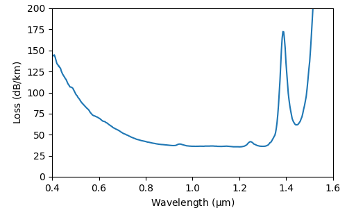
1.4.1. Attenuation of a NLPM750 fiber

This example demonstrates how to use models along with a realistic attenuation profile.

import fmas
import numpy as np
from fmas.grid import Grid
from fmas.models import FMAS_S
from fmas.solver import IFM_RK4IP, SySSM
from ng_fiber_details_nlpm750 import define_alpha_fun_NLPM750


# -- INITIALIZATION STAGE
# ... DEFINE SIMULATION PARAMETERS
t_max = 1000.0  # (fs)
t_num = 2 ** 13  # (-)
z_max = 1.0e5  # (micron)
z_num = 1000  # (-)
z_skip = 10  # (-)
# ... PROPAGGATION CONSTANT
alpha_fun = define_alpha_fun_NLPM750()
# ... COMPUTATIONAL DOMAIN, MODEL, AND SOLVER
grid = Grid(t_max=t_max, t_num=t_num, z_max=z_max, z_num=z_num)
model = FMAS_S(w=grid.w, beta_w=0.0, alpha_w=alpha_fun(grid.w), n2=0.0)
solver = SySSM(model.Lw, model.Nw)

# -- SET UP INITIAL CONDITION
u_0w = np.where(np.logical_and(grid.w > 1, grid.w < 6.0), 1, 0)
solver.set_initial_condition(grid.w, u_0w)

# -- PERFORM Z-PROPAGATION
solver.propagate(z_range=z_max, n_steps=z_num, n_skip=z_skip)

import matplotlib as mpl
import matplotlib.pyplot as plt
import matplotlib.colors as col

f, ax = plt.subplots(1, 1, figsize=(5, 3))
plt.subplots_adjust(left=0.15, right=0.96, bottom=0.15, top=0.96, hspace=0.2)

I0 = np.abs(solver.uwz[0]) ** 2
Iz = np.abs(solver.uwz[-1]) ** 2
_dB = lambda x: 10.0 * np.log10(x)
loss_w = (
    -_dB(
        np.divide(
            Iz,
            I0,
            out=np.ones(grid.w.size, dtype="float"),
            where=I0 > 1e-10,
        )
    )
    * 1e9
    / z_max
)

w = grid.w
w_mask = np.logical_and(w > 1, w < 5.0)
_lam = lambda w: 2 * np.pi * 0.3 / w

ax.plot(_lam(w[w_mask]), loss_w[w_mask])

ax.xaxis.set_ticks_position("bottom")
ax.yaxis.set_ticks_position("left")
ax.set_xlim([0.4, 1.6])
ax.set_ylim([0, 200])
ax.ticklabel_format(useOffset=False, style="sci")
ax.set_xlabel(r"Wavelength $\mathrm{(\mu m)}$")
ax.set_ylabel(r"Loss $\mathrm{(dB/km)}$")

plt.show()