1.4.2. Nonlinear Schrödinger equation with loss

This example demonstrates how to perform simulations for the nonlinear Schrödinger equation including loss.

We first import the functionality needed to perform the sequence of numerical experiments:

import sys
import numpy as np
from fmas.models import ModelBaseClass
from fmas.config import FTFREQ, FT, IFT, C0
from fmas.grid import Grid
from fmas.solver import SySSM

Next, we implement a model for the nonlinear Schrödinger equation. In particular, we here consider the standard nonlinear Schrödinger equation, given by

\[\partial_z u = -\alpha u -i \frac{\beta_2}{2}\partial_t^2 u + i\gamma |u|^2 u,\]

wherein \(u = u(z, t)\) represents the slowly varying pulse envelope, where \(\alpha\) is the root-power attenuation constant accounting for fiber loss, \(\beta_2=-1\) is the second order dispersion parameter, and \(\gamma=1\) is the nonlinear parameter:

class NSE(ModelBaseClass):
    def __init__(self, w, beta, alpha, gamma):
        super().__init__(w, beta_w=beta, alpha_w=alpha)
        self.gamma = gamma

    @property
    def Lw(self):
        return 1j * self.beta_w - self.alpha_w

    def N(self, uw):
        ut = IFT(uw)
        return 1j * self.gamma * FT(np.abs(ut) ** 2 * ut)

Next, we set up the computational domain, the model, an instance of a symmetric split-step Fourier solver and prepare an initial condition given by a fundamental soliton.

To construct the initial condition, we use the exact single-soliton solution of the nonlinar Schrödinger equation, given by

\[u_{\rm{exact}}(z,t) = \sqrt{P_0} {\rm{sech}}(t/t_0)\,e^{-i\gamma P_0 z/2},\]

with \(P_0=|\beta_2|/(\gamma t_0^2)\). We here consider a fundamental soliton of duration \(t_0=1\) and use \(u_{\rm{exact}}(0,t)\) as initial condition. The propagation is performed up to \(z_{\rm{max}}=\pi/2\), i.e. for one soliton period.

# -- SET MODEL PARAMETERS
t_max = -50.0
Nt = 2 ** 12
# ... PROPAGATION CONSTANT (POLYNOMIAL MODEL)
b2 = -1.0
beta = lambda w: 0.5 * b2 * w * w
# ... NONLINEAR PARAMETER
gamma = 1.0
# ... POWER ATTENUATION PARAMETER
alpha = 1.0
# ... SOLITON PARAMTERS
t0 = 1.0  # duration
P0 = np.abs(b2) / t0 / t0 / gamma  # peak-intensity
LD = t0 * t0 / np.abs(b2)  # dispersion length
# ... EXACT SOLUTION
u_exact = lambda z, t: np.sqrt(P0) * np.exp(0.5j * gamma * P0 * z) / np.cosh(t / t0)

We here measure the effect of fiber loss by monitoring the energy

\[E(z) = \sum_w |u_\omega(z)|^2\]

which is expected to decay as

\[E(z) = E(0)\,e^{-2 \alpha z}\]

def Ce(i, zi, w, uw):
    return np.sum(np.abs(uw) ** 2)


# -- INITIALIZATION STAGE
# ... COMPUTATIONAL DOMAIN
grid = Grid(t_max=t_max, t_num=Nt)
t, w = grid.t, grid.w

model = NSE(w, beta(w), alpha, gamma)
# ... PROPAGATION ALGORITHM
solver = SySSM(model.Lw, model.N, user_action=Ce)
# ... INITIAL CONDITION
solver.set_initial_condition(w, FT(u_exact(0.0, t)))

# -- RUN SOLVER
solver.propagate(z_range=0.5 * np.pi * LD, n_steps=512, n_skip=2)  # propagation range

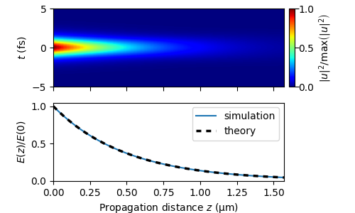
In the figure below, the top subfigure shows the time-domain propagation dynamics of a fundamental soliton for the nonlinear Schrödinger equation in the presence of fiber loss. The subfigure at the bottom show the resulting decay of the energy in the numerical experiment (solid line), along with the theoretical prediction (dashed line).

import matplotlib as mpl
import matplotlib.pyplot as plt
import matplotlib.colors as col

f, (ax1, ax2) = plt.subplots(2, 1, figsize=(5, 3))
plt.subplots_adjust(left=0.15, right=0.8, bottom=0.15, top=0.96, hspace=0.2)
cmap = mpl.cm.get_cmap("jet")


def _setColorbar(im, refPos):
    """colorbar helper"""
    x0, y0, w, h = refPos.x0, refPos.y0, refPos.width, refPos.height
    cax = f.add_axes([x0 + 1.02 * w, y0, 0.025 * w, h])
    cbar = f.colorbar(im, cax=cax, orientation="vertical")
    cbar.ax.tick_params(
        color="k",
        labelcolor="k",
        bottom=False,
        direction="out",
        labelbottom=False,
        labeltop=True,
        top=True,
        size=4,
        pad=0,
    )
    cbar.ax.tick_params(which="minor", bottom=False, top=False)
    return cbar


# -- TOP SUB-FIGURE: TIME-DOMAIN PROPAGATION CHARACTERISTICS
It = np.abs(solver.utz) ** 2
It /= np.max(It)

im1 = ax1.pcolorfast(
    solver.z,
    grid.t,
    np.swapaxes(It[:-1, :-1], 0, 1),
    norm=col.Normalize(vmin=0, vmax=1),
    cmap=cmap,
)
cbar1 = _setColorbar(im1, ax1.get_position())
cbar1.ax.set_ylabel(r"$|u|^2/{\rm{max}}\left(|u|^2\right)$")
ax1.xaxis.set_ticks_position("bottom")
ax1.yaxis.set_ticks_position("left")
ax1.set_ylim(-5, 5)
ax1.set_xlim([0.0, solver.z.max()])
ax1.set_ylabel(r"$t~\mathrm{(fs)}$")
ax1.ticklabel_format(useOffset=False, style="plain")
ax1.tick_params(axis="x", labelbottom=False, length=4)

# -- BOTTOM SUB-FIGURE: ENERGY DECAY
Ez = lambda z: solver.ua_vals[0] * np.exp(-2*alpha * z)
ax2.plot(solver.z, solver.ua_vals / Ez(0), lw=1.5, label="simulation")
ax2.plot(
    solver.z, Ez(solver.z) / Ez(0), color="k", lw=2.5, dashes=[2, 2], label="theory"
)
ax2.xaxis.set_ticks_position("bottom")
ax2.yaxis.set_ticks_position("left")
ax2.set_xlim([0.0, solver.z.max()])
ax2.ticklabel_format(useOffset=False, style="sci")
ax2.set_xlabel(r"Propagation distance $z~\mathrm{(\mu m)}$")
ax2.set_ylabel(r"$E(z)/E(0)$")
ax2.legend()

plt.show()