1.1.2. Basic workflow

This examples demonstrates a basic workflow using the py-fmas library code.

We start by simply importing the required fmas into the current namespace.

import fmas

If an adequate input file is located within the current working directory, the function read_h5, located in module data_io, can be used to read-in the propagation setting stored in the input file input_file.h5:

glob = fmas.data_io.read_h5('input_file.h5')

Next, the problem specific data structures, given by the computational grid and the propagation model, can be initialized:

grid = fmas.grid.Grid(
    t_max = glob.t_max,
    t_num = glob.t_num,
    z_max = glob.z_max,
    z_num = glob.z_num)

model = fmas.models.FMAS_S_R(
    w = grid.w,
    beta_w = glob.beta_w,
    n2 = glob.n2,
    fR = glob.fR,
    tau1 = glob.tau1,
    tau2 = glob.tau2)

The provided initial condition, which represents the real-valued optical field can be converted to the complex-valued analytic signal as shown below:

ic = fmas.analytic_signal.AS(glob.E_0t)

Below we implement a user-action function that can be passed to the propagation algorithm. Upon propagation it will evaluated at every \(z\)-step

import numpy as np

def Cp(i, zi, w, uw):
    Iw = np.abs(uw)**2
    return np.sum(Iw[w>0]/w[w>0])

Next, we initialzize the \(z\)-propagation algorithm, given by the Runge-Kutta in the interaction picture (RK4IP) method, set the initial condition, and perform \(z\)-propagation:

solver = fmas.solver.IFM_RK4IP(
    model.Lw, model.Nw,
    user_action = Cp)

solver.set_initial_condition(
    grid.w, ic.w_rep)

solver.propagate(
    z_range = glob.z_max,
    n_steps = glob.z_num,
    n_skip = glob.z_skip)

After the propagation algorithm has terminated, the generated simulation data can be stored within an output file in HDF5-format. Therefore, the data is organized as dictionary with custom keys for the stored data objects, which is then passed to the function save_h5 implemented in module data_io:

res = {
    "t": grid.t,
    "z": solver.z,
    "w": solver.w,
    "u": solver.utz,
    "Cp": solver.ua_vals}

fmas.data_io.save_h5('out_file.h5', **res)

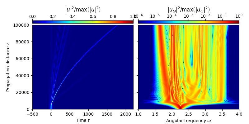
A simple plot of the generated data can be obtained using convenience functions implemented in module tools:

fmas.tools.plot_evolution(
    solver.z, grid.t, solver.utz,
    t_lim = (-500,2200), w_lim = (1.,4.))